Decomposing supply shocks in the US electricity industry: evidence from a time-varying Bayesian panel vector autoregression model

Nicholas Apergis; Michael Polemis

1 Introduction

There is a general consensus among researchers and practitioners that the electricity industry constitutes one of the most important energy sectors in the United States, with a net generation of 4078 terawatt-hours in 2015 and retail sales equal to 3711 billion kilowatt-hours (International Energy Agency 2019). The industry is also crucial for the competitiveness and economic growth of the US economy, since it has an impact on all other economic activities.

The reliability and quality of electricity supply are, however, vulnerable to shocks (disruptions) generated either from external factors such as natural disasters (eg, droughts, earthquakes) or from human activity (eg, nuclear accidents). Specifically, the tsunami in Fukushima in 2011, which was initiated by an earthquake, is a typical example of a natural disaster. However, this caused an accident in the nuclear power plant immediately after the event as the active reactors automatically shut down their sustained fission reactions, causing extended power supply shortages. This resulted in persistent electricity price hikes, due to the shutdown of a large number of nuclear power plants for safety checks in light of the accident. Moreover, the electricity crisis that hit Ecuador in 2009, stimulated by a severe drought that depleted water levels at hydroelectric plants, is another striking example of supply-side electricity distortions that led to extensive brownouts and power supply cuts affecting the performance of the whole economy. Finally, we cannot fail to notice that the California electricity crisis, dating back to 2000, constitutes another example of electricity supply shortage, triggered by market manipulations, shutdowns of pipelines by Enron and capped retail electricity prices. This event had a significant macroeconomic impact on the US economy, in addition to market structure distortions, such as price spikes, capacity manipulation and megawatt laundering (Joskow 2001; Joskow and Kohn 2002). Even though such shocks occur rather infrequently, they can cause considerable socioeconomic costs and consequences across the whole spectrum of economic activity (Poudineh and Jamasb 2017; Levine et al 2005). In other words, electricity supply interruptions result in shock transmissions and spillover (cascading) effects to other sectors of the economy (Poudineh and Jamasb 2017; Giulietti et al 2010).

Although there is growing research activity on the impact of oil supply shocks on the main macroeconomic variables such as the level of economic growth or employment (see, for example, Barsky and Kilian 2002; Hamilton 2003; Ramey and Vine 2011; Kilian 2008a,b, 2009a,b), little attention has been paid to the macroeconomic consequences of electricity supply shocks. This study aims to fill this gap in the literature by decomposing the main drivers of the electricity supply shocks by the type of fuel used in the generation process. Specifically, the issue of electricity supply shocks has been researched recently for developing countries in particular (eg, Chile, South Africa), where extended power cuts and load shedding lead to serious and systematic power interruptions. This strand of the literature is growing rapidly and calls for an in-depth examination from both a theoretical and an empirical standpoint (Allcott et al 2016; Hunt et al 2016; Andersen and Dalgaard 2013; Cheng et al 2013).

Poudineh and Jamasb (2017) apply an extensive (Leontief-type) input–output model to investigate the impact of electricity supply shocks on the performance of 101 sectors of the Scottish economy, in tandem with the estimation of the societal cost of energy not supplied (SCENS) due to an interruption. They claim that inoperability corresponds to a heterogeneous level of economic losses across all the sectors of economic activity investigated. Also, their empirical findings postulate that SCENS varies with the duration of a power cut.¹¹ 1 We stress that the estimation of SCENS due to electricity interruptions is beyond the scope of this paper. However, a detailed review of interruption costs studies can be found in Toba (2007).

Our approach deviates from the existing literature, which focuses solely on the examination of electricity supply interruptions from a microeconomic perspective (Reichl et al 2013; de Nooij et al 2007; Balducci et al 2002). Specifically, our study constitutes one of the very few attempts at modeling and estimating the determinants of possible electricity supply shocks on the macroeconomic performance of a large-scale economy, such as the United States. More specifically, the empirical methodology adopted in this paper makes use of modeling the gross domestic product (GDP) per capita growth across US states over time in vector autoregressive (VAR) models by allowing the coefficients to vary stochastically, while they are also free to vary as a deterministic function of observable economic characteristics, such as total electricity supply or other economic controls, typically obtained by pooling the data across US states and time in a panel VAR set up for that purpose.

The aim of this paper is to investigate the relationship and the possible spillovers between electricity supply shocks and US macroeconomic performance, since there is considerable evidence that this relationship is unstable over time. Our analysis uses monthly regional data from the US states, spanning the period from January 2001 to September 2016, and combines a novel identification strategy for electricity supply shocks based on inequality constraints with the estimation of a time-varying Bayesian panel VAR model (TVBPVAR). This methodology makes use of a Bayesian shrinkage estimator for panel VAR models which, unlike time series VAR modeling, also allows the coefficients to vary as a stochastic function of the observable characteristics (Wieladek 2016).

The contribution of this paper is fourfold. First and foremost, it attempts to link the electricity supply shocks decomposed by fuel mix (ie, nuclear, coal, renewable energy sources, natural gas, etc) with US macroeconomic performance. Given that the electricity system is comprised of generation (different sources), transmission and distribution (end-user), the fuel mix may be important, as it addresses electrical power (measured by nameplate capacity and plant utilization), while electrical energy is the product and is essentially a commodity (and thus perfectly substitutable). In that sense, this study controls for shocks that may have differential effects because plant utilization (for given nameplate capacity) differs dramatically by source (for example, plant utilization is much lower for wind and solar than it is for a natural gas electricity generation). Our finding that source (fuel mix) shocks do not differ suggests that the system is operating (near) optimally, in that transmission and distribution are not affected by the source of the shock. Thus, it is the increased electrical supply that matters for macro growth. We attempt to shed some light on the mechanism of electricity supply shocks and how these shocks have changed over time.

Second, the empirical model allows for time-varying heteroscedasticity in the VAR innovations, which accounts for changes in the magnitude of structural shocks and their immediate impact on US macroeconomic performance.

Third, it goes beyond the existing literature in that it uses a particularly long panel of forty-eight US states on a monthly basis over the period from January 2001 to September 2016.

Finally, in contrast to existing empirical studies that assume the variables are not correlated across the panel dimension (cross-section independence), we perform appropriate techniques to deal with this issue. This is a common occurrence in macrolevel data, resulting in low power and size distortions in tests that assume cross-section independence (Pesaran 2004). The latter may arise due to common unobserved effects caused by changes in the US states’ legislation (taxation, currency regulatory restrictions, import quotas, etc).

The rest of the paper is organized as follows. Section 2 describes the electricity industry in the United States, focusing on the supply and demand conditions across the regions (states), along with the existing regulatory and competitive framework. Section 3 describes the data and performs the necessary preliminary testing (ie, cross-section dependence test, unit root and cointegration testing). Section 4 presents the empirical methodology, while Section 5 illustrates the empirical findings. Section 6 performs the necessary robustness checks to strengthen the validity of the empirical findings. Lastly, Section 7 states the conclusions of the paper, providing some policy recommendations.

2 The electricity industry in the United States

The electricity industry in the United States is made up of over 3000 public, private and cooperative utilities, including more than 1000 independent power producers, three regional synchronized power grids, eight electricity reliability councils, some 150 control-area operators and thousands of separate engineering, economic, environmental and land-use regulatory authorities (International Energy Agency 2014). The power supply is generated from a diverse fuel mix. Specifically, fossil fuels (ie, coal, natural gas and petroleum liquids) account for 67% of US electricity generation and 89% of installed capacity (International Energy Agency 2014). Generation capacity also varies by state and can be dependent upon the availability of fuel resources. Coal and gas power plants are more common in the Midwest and Southeast, whereas the West Coast is dependent upon high-capacity hydroelectric power as well as gas-fired power plants (International Energy Agency 2014). Power generation fuels also have a supply chain of their own. Coal, natural gas, uranium and oil must all be extracted, processed into useable fuels and delivered to the generation facility. Vast infrastructure networks of railroads, pipelines, waterways, highways and processing plants all support the delivery of these resources to generating facilities, and many rely on electric power to operate (US Department of Energy 2015).²² 2 The United States Electricity Industry Primer provides a high-level overview of the US electricity supply chain, including the generation, transmission and distribution process; markets and ownership structures, including utilities and regulatory agencies; and system reliability and vulnerabilities.

Over the last ten years, the proportion of renewables in the energy mix has increased. Nevertheless, fossil fuels (primarily oil, natural gas and coal) are still the predominant sources of energy consumption in the country. It is expected that renewable capacity will continue to increase under pressure from a public concerned with climate change and improvements in renewable technologies and costs (International Energy Agency 2014).

It is worth mentioning that the electricity industry is regulated by both state and federal regulatory bodies. The Federal Energy Regulatory Commission (FERC) enjoys exclusive jurisdiction over the transmission of electricity in interstate commerce, the wholesale sale of electric energy in interstate commerce and the overall facilities for such transmission or sales of electric energy (International Energy Agency 2014). The FERC also has jurisdiction over wholesale transactions where there is no crossing of state boundaries. Specifically, it regulates both the wholesale electricity markets and interstate transmission services (market structure, transmission planning and cost allocation, bulk power system reliability, etc). In contrast, state utility commissions regulate issues such as retail rates and distribution services, distribution rates across all states, supply rates (integrated states) or default service procurements and retail choice rules (restructured states), resource planning/adequacy, generation and transmission siting, demand-side resources and distribution reliability. The North American Electric Reliability Corporation (NERC) is a regulatory authority whose mission is to ensure the reliability and security of the bulk power system in North America (United States, Canada, Mexico). Specifically, NERC develops and enforces reliability standards; it annually assesses seasonal and long-term reliability and monitors the bulk power system through system awareness. The NERC is the electric regulatory organization for North America, subject to oversight by the FERC and governmental authorities in Canada. The NERC’s jurisdiction includes users, owners and operators of the bulk power system, serving more than 334 million people.

Most US states follow a “regulated” model, but many are “restructured”. Specifically, in regulated states, utilities are vertically integrated and prepare integrated resource plans to serve their load. Supply and distribution rates are set through economic regulation. In restructured states, generation is deregulated and supply rates are set by the markets. Distribution services are still fully regulated, and distribution rates are set through economic regulation. It is worth mentioning that restructured utilities do not prepare integrated resource plans, but states retain some authority over direct generation and demand-side resources. Overall, the (de)regulation of the electricity industry still varies by state.

Finally, the electricity industry in the United States includes industry players that provide a wide range of both privately and publicly owned services. Generally, in the southeastern, southwestern and northwestern states, electric utilities are responsible for the operation and maintenance of the electricity system, providing retail customers with electrical power. The majority of these utilities are vertically integrated, where they own the systems responsible for the generation, transmission and distribution of electricity. Most utilities are publicly owned, although there are about ten federal utilities.

3 Data and preliminary empirical testing

3.1 Data description

Our empirical analysis is based on a large panel data set of 9072 monthly observations, spanning the period from January 2001 to September 2016 ( $N=48$ and $T=189$ ). The selected sample includes forty-eight US states, with Alaska and Hawaii being omitted. The starting date for the study was dictated by energy data availability, while the final date observation (September 2016) represents the last month for which data mostly regarding the US Energy Information Administration (EIA) was available at the time the research was conducted.

The electricity supply variables are seasonally adjusted and include both total electricity generation (per capita) and power production by specific energy sources (coal, nuclear, natural gas, oil, hydroelectric, biomass, wind and solar). The reason for decomposing electricity generation by fuel is to investigate whether different patterns of electricity supply shocks prevail in the industry and thus affect the overall macroeconomic performance of the US economy. All the above variables are primarily taken from the EIA electricity data browser.³³ 3 See http://www.eia.gov/electricity/data/browser/. The level of economic growth is proxied by per capita real GDP across US states (measured in 2009 US dollars). The latter, which is drawn from the regional economic accounts of the Bureau of Economic Analysis (BEA), provides the market value of goods and services produced by the labor and property located in a US state.⁴⁴ 4 See http://www.bea.gov/regional/index.htm. In other words, real GDP by state is an inflation-adjusted measure based on national prices for the goods and services produced within each state. Total employment (full-time and part-time) is used as a proxy for the labor force. The total employment variable, which is also taken from the BEA, includes wage and salary jobs and sole proprietorships over the sample period, but not unpaid family workers or volunteers per US state. School enrolment is used as a proxy for human capital and includes secondary school enrolment. This variable is drawn primarily from the National Center for Education Statistics at the US Department of Education. Gross fixed capital formation includes the following:

•

land improvements;
•

plant, machinery and equipment purchases;
•

construction of roads, railways, etc;
•

construction of schools, offices, hospitals, private residential dwellings, commercial and industrial buildings; and
•

net acquisitions of valuables.

This indicator is measured in constant 2010 US dollar prices per US state and is extracted from the Datastream database. Moreover, we use the public deficit variable drawn primarily from the Federal, State and Local Governments database from the US Census Bureau of the US Department of Commerce.⁵⁵ 5 See http://www.census.gov/govs/.

In the case of the US states, the analysis also uses the following variables.

(1)

Trade openness, defined as the ratio of the sum of exports and imports to GDP (data sourced from the BEA).
(2)

The total population of the state (mid-year estimate) (data sourced from the US Census Bureau).
(3)

Urbanization, defined as the percentage of population living in urban areas (data sourced from the US Census Bureau).
(4)
The shares of total earnings (data obtained from the BEA) in
1. (a)
  
  “farm” and “other agriculture” industries (in thousands, including net farm proprietors’ income and the wages and salaries, pay-in-kind and supplements to wages and salaries of hired farm laborers),
2. (b)
  
  “manufacturing” industries (in thousands, including establishments engaged in the mechanical or chemical transformation of materials or substances into new products,⁶⁶ 6 These establishments are usually described as plants, factories or mills and characteristically use power-driven machines and materials-handling equipment. establishments engaged in assembling component parts of manufactured products if the new product is neither a structure nor other fixed improvement, and establishments engaged in the blending of materials, such as lubricating oils, plastics resins or liquors) and
3. (c)
  
  “service” industries (in thousands, including establishments primarily engaged in providing a wide variety of services for individuals, business and government establishments, and other organizations; hotels and other lodging places; establishments providing personal, business, repair and amusement services; health, legal, engineering and other professional services; educational institutions; membership organizations and other miscellaneous services).

Table 1: Summary statistics for the sample variables. [The table reports summary statistics for the forty-eight US states in the sample over the period from January 2001 to September 2016. All variables are used as natural logarithms in the econometric analysis (when appropriate). SD denotes standard deviation.]

Variable	Mean	SD	Min	Max
Per capita GDP	0 043 648.3	013 279.9	$-$ 029 957	00 070 918
Total electricity supply	0 006 384.4	005 759.3	$-$ 000 025	00 044 280
Electricity from coal	0 002 943	002 963	000 00 $-$ 6	00 015 815
Electricity from nuclear	0 001 315.5	001 715.9	000 0 $-$ 26	00 008 871
Electricity from natural gas	0 001 428.2	002 647.5	$-$ 000 000	00 022 893
Electricity from oil	0 000 097.1	000 329.9	000 0 $-$ 18	00 005 296
Electricity from wind	0 000 139	000 380	$-$ 000 000	00 005 670
Electricity from solar	0 000 009.58	000 080.6	$-$ 000 000	00 002 190
Hydroelectric electricity	0 000 429.3	001 078.4	000 $-$ 248	00 011 209
Biomass electricity	0 000 043.7	000 070.4	000 00 $-$ 1	00 000 640
Labor force	5 955 590	425 580.1	$-$ 330 154	46 257 210
Gross capital formation	0 000 718.7	000 082.0	$-$ 000 586.2	00 000 862.4
Public deficit (%)	0 000 012.2	000 000.0045	$-$ 000 011.4	00 000 013.1
School enrolment	0 958 965	094 142.1	$-$ 068 681	06 742 400
Trade openness	0 000 026.5	000 004.39	$-$ 000 022.4	00 000 033.9
State population	6 201 127	179 466.7	$-$ 564 513	39 250 017
Urbanization (%)	0 000 084.5	000 005.9	$-$ 000 077.6	00 000 088.9
Share of total earnings:
from agriculture	0 609 747	242 848	$-$ 529 365	08 500 946
from manufacturing	9 106 320	344 216	$-$ 033 593	13 099 461
from services	1 145 682	339 895	$-$ 070 591	27 890 673

Table 1 reports a set of descriptive statistics for all the variables used in the empirical analysis. It is evident from the table that the data is well behaved, showing limited variability concerning the mean of the population, since the coefficient of variation does not exceed 50% in all cases. On the other hand, as expected, the variables do not follow the normal distribution, since the relative values of the skewness and kurtosis measures are not $0$ and $3$ , respectively.

3.2 Preliminary testing for cross-section dependence and unit roots

In the first step of our empirical analysis, we examine the unit root properties in the data through advanced panel unit root tests. First-generation panel unit root tests can lead to spurious results (because of size distortions) if significant degrees of positive residual cross-section dependence exist and are ignored. Consequently, the implementation of second-generation panel unit root tests is desirable only when it has been established that the panel is subject to a significant degree of residual cross-section dependence. In the cases where cross-section dependence is not sufficiently high, a loss of power might result if second-generation panel unit root tests that allow for cross-section dependence are employed. Therefore, before selecting the appropriate panel unit root test, it is crucial to provide some evidence on the degree of residual cross-section dependence.

The cross-section dependence (CD) statistic by Pesaran (2004) is based on a simple average of all pairwise correlation coefficients of the ordinary least squares residuals obtained from standard augmented Dickey–Fuller (ADF) regressions for each variable in the panel. Under the null hypothesis of cross-section independence, the CD test statistic asymptotically follows a standard normal distribution. The test is based on the estimation of a linear panel model of the form

y_{it}=\alpha_{i}+\beta_{i}^{\prime}x_{it}+u_{it},\quad i=1,\dots,N,~{}t=1,% \dots,T,

(3.1)

where $T$ and $N$ are the time and panel dimensions, respectively, $\alpha_{i}$ is the province-specific intercept, $x_{it}$ is a $k\times 1$ vector of regressors and $u_{it}$ is the random disturbance term. The null hypothesis assumes the existence of cross-sectional correlation: $\operatorname{cov}(u_{it},u_{jt})=0$ for all $t$ and all $i\neq j$ . This is tested against the alternative hypothesis that $\operatorname{cov}(u_{it},u_{jt})\neq 0$ for at least one pair of $i$ and $j$ .

The cross-section dependence test results uniformly reject the null hypothesis of cross-section independence, providing evidence of cross-section dependence in the data given the statistical significance of the CD statistics regardless of the number of lags (from 1 to 4) included in the ADF regressions.

A second-generation panel unit root test is employed to determine the degree (order) of integration in the respective variables. The Pesaran (2007) panel unit root test (also known as the crossâsectionally augmented Im–Pesaran–Shin (CIPS) test) does not require the estimation of factor loading to eliminate cross-section dependence. Specifically, the usual Dickey–Fuller regression is augmented to include the lagged cross-sectional mean and its first difference to capture the cross-section dependence that arises through a single-factor model. The null hypothesis is a unit root for the Pesaran (2007) test. The CIPS test is based on the cross-sectional ADF test as follows:

\Delta y_{it}=\alpha_{i}+\rho_{i}y_{i,t-1}+\beta_{i}\bar{y}_{t-1}+c_{i}\Delta% \bar{y}_{t}+u_{it},

(3.2)

where

\bar{y}_{t-1}=n^{-1}\sum_{i=1}^{n}y_{i,t-1}\quad\text{and}\quad\Delta y_{t}=n^% {-1}\sum_{i=1}^{n}\Delta\bar{y}_{t}

are used as proxies for the effect of the unobserved common factor. The CIPS test statistic is simply the average $t$ -statistic of the ordinary least squares estimate for $\rho_{i}$ for the individual sections. The null hypothesis that $\rho_{i}=0$ for all $i$ is tested against the alternative that only fractions of the series are stationary. The results are reported in Table 2 and support the presence of a unit root across all the variables under consideration. In other words, our sample variables are integrated of order 1 ( $I(1)$ ).

Table 2: Panel unit root test. [

\Delta

denotes first differences. A constant is included in the Pesaran (2007) tests. Rejection of the null hypothesis indicates stationarity in at least one country. CIPS

{}^{*}

denotes the truncated CIPS test. Critical values for the Pesaran (2007) test are

-

2.40 at 1%,

-

2.22 at 5% and

-

2.14 at 10%, respectively. The results are reported at

\text{lag}=\text{4}

. The null hypothesis is that of a unit root.

{}^{***}

denotes

p\leq\text{0.01}

.]

Variable	Pesaran (CIPS)	Pesaran (CIPS ${}^{*}$ )
Per capita GDP	$-$ 1.28	$-$ 1.33
$\Delta$ per capita GDP	$-$ 6.31 ${}^{***}$	$-$ 6.57 ${}^{***}$
Electricity supply	$-$ 1.38	$-$ 1.42
$\Delta$ electricity supply	$-$ 6.14 ${}^{***}$	$-$ 6.30 ${}^{***}$
Electricity from coal	$-$ 1.25	$-$ 1.34
$\Delta$ electricity from coal	$-$ 5.79 ${}^{***}$	$-$ 5.96 ${}^{***}$
Electricity from nuclear	$-$ 1.36	$-$ 1.40
$\Delta$ electricity from nuclear	$-$ 5.80 ${}^{***}$	$-$ 5.96 ${}^{***}$
Electricity from natural gas	$-$ 1.27	$-$ 1.33
$\Delta$ electricity from natural gas	$-$ 6.13 ${}^{***}$	$-$ 6.25 ${}^{***}$
Electricity from oil	$-$ 1.32	$-$ 1.38
$\Delta$ electricity from oil	$-$ 6.42 ${}^{***}$	$-$ 6.69 ${}^{***}$
Electricity from wind	$-$ 1.39	$-$ 1.44
$\Delta$ electricity from wind	$-$ 5.89 ${}^{***}$	$-$ 6.06 ${}^{***}$
Electricity from solar	$-$ 1.27	$-$ 1.35
$\Delta$ electricity from solar	$-$ 6.10 ${}^{***}$	$-$ 6.28 ${}^{***}$
Hydroelectric electricity	$-$ 1.36	$-$ 1.41
$\Delta$ hydroelectric electricity	$-$ 5.84 ${}^{***}$	$-$ 6.01 ${}^{***}$
Biomass electricity	$-$ 1.36	$-$ 1.40
$\Delta$ biomass electricity	$-$ 5.92 ${}^{***}$	$-$ 6.10 ${}^{***}$
Labor force	$-$ 1.22	$-$ 1.29
$\Delta$ labor force	$-$ 6.27 ${}^{***}$	$-$ 6.39 ${}^{***}$
Gross capital formation	$-$ 1.25	$-$ 1.31
$\Delta$ gross capital formation	$-$ 6.12 ${}^{***}$	$-$ 6.24 ${}^{***}$
Public deficit	$-$ 1.28	$-$ 1.36
$\Delta$ public deficit	$-$ 6.19 ${}^{***}$	$-$ 6.30 ${}^{***}$
School enrollment	$-$ 1.33	$-$ 1.39
$\Delta$ school enrollment	$-$ 5.87 ${}^{***}$	$-$ 6.03 ${}^{***}$
Trade openness	$-$ 1.28	$-$ 1.35
$\Delta$ trade openness	$-$ 5.68 ${}^{***}$	$-$ 5.93 ${}^{***}$
State population	$-$ 1.32	$-$ 1.39
$\Delta$ state population	$-$ 5.77 ${}^{***}$	$-$ 5.96 ${}^{***}$
Urbanization	$-$ 1.26	$-$ 1.34
$\Delta$ urbanization	$-$ 5.94 ${}^{***}$	$-$ 6.25 ${}^{***}$
Share of total earnings from agriculture	$-$ 1.31	$-$ 1.38
$\Delta$ share of total earnings from agriculture	$-$ 5.62 ${}^{***}$	$-$ 5.85 ${}^{***}$
Share of total earnings from manufacturing	$-$ 1.26	$-$ 1.33
$\Delta$ share of total earnings from manufacturing	$-$ 5.83 ${}^{***}$	$-$ 6.17 ${}^{***}$
Share of total earnings from services	$-$ 1.30	$-$ 1.38
$\Delta$ share of total earnings from services	$-$ 5.69 ${}^{***}$	$-$ 5.94 ${}^{***}$

4 Empirical methodology

The literature has recorded several studies in estimating VAR models with time-varying coefficients. Such studies explore the transmission mechanism of monetary policy (see, for example, Cogley and Sargent 2005) and fiscal policy (Pereira and Lopes 2010) to shocks on output and inflation, while other studies make use of these methods (ie, the Bayesian time-varying vector error correction and seasonal autoregressive integrated moving average models) to forecast electricity demand (Grasso 2010). Moreover, Hurn et al (2016) employ a smooth transition logit model to detect the presence of potential structural changes in the electricity industry stemming from deregulation. The model allows the timing of any change to be determined endogenously and also the market participants’ behavior to change gradually over time. Their main empirical findings indicate the presence of a structural change, consistent with the process of deregulation in Australia. Most papers in this literature assume that coefficients evolve stochastically according to a slowly moving random walk, implying that changes in the coefficients can reflect permanent structural changes. However, it is not possible to infer why such structural changes occur.

A different strand of the literature has related changes in the transmission of shocks to certain observable economic characteristics (Mertens 2008; Olivei and Tenreyro 2007, 2010). Assenmacher-Wesche and Gerlach (2010) and Calza et al (2013) estimate panel VAR models on sets of countries with developed and less developed financial markets to infer the impact of the mortgage market development on the monetary policy transmission mechanism. If the economic characteristic in question can be observed both over time and cross-sectionally, it might, of course, be more desirable to estimate a model that exploits all of the variations across both of these dimensions. However, to the best of our knowledge, no study has applied this methodological approach to explore the link between economic growth and electricity supply across the US states. Let us assume the following time-varying coefficient panel VAR model:

Y_{c,t}=X_{c,t}B_{c}+E_{c,t}\quad\text{with }E_{c,t}\sim\Big{(}0^{\prime}_{c,t% },\sum cA_{c,t}\Big{)},

(4.1)

where $Y_{c,t}$ is a $1\times N$ matrix of $N$ endogenous variables for state $c$ at time $t$ containing the lags of $Y_{c}$ and a constant term. Based on the work by Wieladek (2016) (in which the mathematical details of the model can be found), it is assumed that these coefficients vary as a function of the observables:

	$\displaystyle\beta_{c}\mid y_{c,t}X_{c,t}a_{c,t}\sum c$	$\displaystyle\sim N(D_{c,t}\delta_{\beta},\varLambda_{BC}),$		(4.2)
	$\displaystyle\alpha_{c}\mid y_{c,t}X_{c,t}\beta_{c,t}\sum c$	$\displaystyle\sim N(D_{c,t}\delta_{A},\varLambda_{AC}),$		(4.3)

where $(\delta_{B},\delta_{A})$ is a matrix of pooled coefficients across states, which relate the weakly exogenous variables $D_{c,t}$ to the individual state coefficients $\beta_{c,t}$ , $A_{c,t}$ , with the variances $\varLambda_{BC}$ , $\varLambda_{AC}$ determining the tightness of these priors (Liu et al 2017; Hong and Lian 2012). For our empirical analysis, we estimate this model by repeatedly drawing from the posteriors of the Gibbs sampling chain 150 000 times, discarding the first 50 000 draws as burn-in and retaining every hundredth draw of the remaining draws for inference.

5 Baseline results and discussion

The next step of the baseline empirical analysis involves bivariate time-varying panel VAR modeling in which the GDP per capita and the total supply of electricity are the two endogenous variables involved. Panel VAR models are built with the same logic as standard VAR models and they can be regarded as a much more powerful tool to address interesting policy implications (Canova and Ciccarelli 2013; Polemis 2016). In a panel-VAR framework, all variables are treated as endogenous and interdependent, both in a dynamic sense and in a static sense. Further, one of its major advantages is that it examines the underlying dynamic relationships, unlike the static results generated by fixed-effects models (Mamatzakis et al 2013). The Bayesian panel-VAR framework allows the examination of the impact of electricity supply shock innovations (total electricity generation or decomposed by fuel mix) on the US macroeconomic performance (proxied by the GDP per capita growth indicator) in more detail and is included in this study to perform a sensitivity analysis. However, Kilian and Murphy (2013) argue that it is important to identify the potential simultaneous impacts of electricity supply and electricity demand shocks on economic growth through the imposition of certain quantity restrictions. To this end, we impose the condition that the relevant individual state output is positive if faced with an electricity supply shock and negative if an electricity demand shock prevails.

In particular, the baseline analysis uses a bivariate identification scheme with GDP per capita growth ordered first. Within this methodological framework, it is possible to examine how the coefficients of GDP per capita growth (and the implied impulse responses) are affected by total electricity supply in the following manner: first, evaluate the structural characteristic of interest, ie, total electricity supply, at a high value (defined as the ninetieth percentile of values realized in the sample) to obtain draws of $\beta_{c,t}^{e-1}$ and $a_{c,t}^{e-1}$ , the associated distribution of impulse responses, where $e$ denotes the total electricity supply. Next, we repeat the previous step, but this time with a low value of $e$ (defined as the tenth percentile) to obtain draws of $\beta_{c,t}^{e-2}$ and $a_{c,t}^{e-2}$ . A comparison of these two distributions, subject to the same size shock, allows us to infer the effect of total electricity supply on GDP per capita shocks.

Figure 1 shows the impulse response functions (IRFs) for GDP per capita growth to shocks in total electricity supply (bivariate model) at the tenth percentile and at the ninetieth percentile of total electricity supply. These results illustrate that GDP per capita growth increases following a positive electricity supply shock (across all three distributions), which is a result consistent with a number of time series and panel data studies in the literature (see, for example, Narayan et al 2010; Lorde et al 2010; Bildirici et al 2012; Solarin and Shahbaz 2013; Jakovac and Vlahinić Lenz 2016).

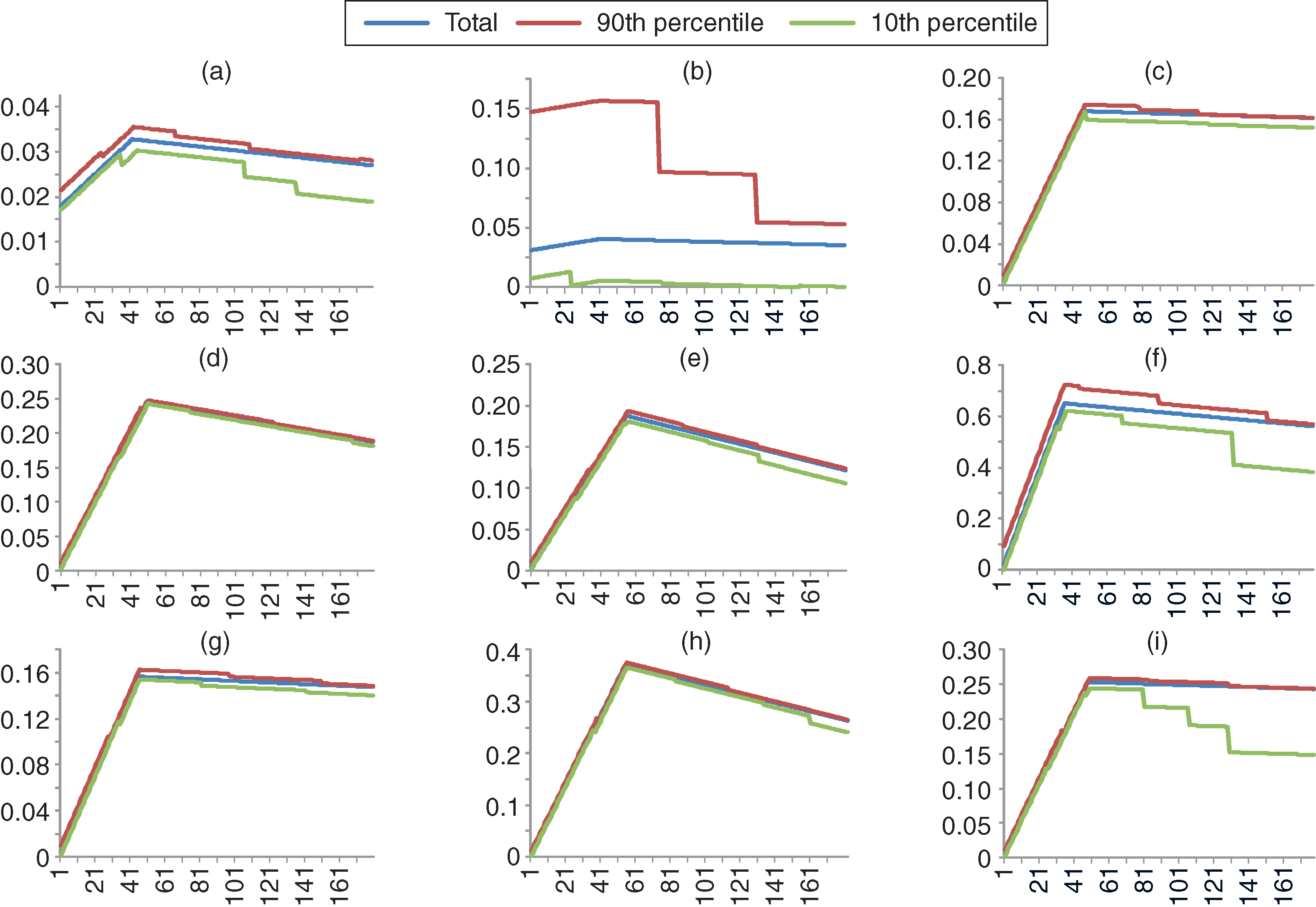
Figure 1: Impulse response functions for the bivariate time-varying Bayesian panel VAR model. (a) Total electricity. (b) Electricity from coal. (c) Electricity from nuclear. (d) Electricity from natural gas. (e) Electricity from oil. (f) Electricity from hydro. (g) Electricity from biomass. (h) Electricity from solar. (i) Electricity from wind. Horizontal axis shows time in months.

Figure 1 also illustrates IRFs for GDP per capita growth to shocks in electricity generated by different fuels (coal, nuclear, natural gas, oil, hydro, biomass, solar, wind). The new empirical findings support the notion that decomposed electricity shocks have a robust positive impact on GDP per capita growth, indicating that all sources of energy seem to be conducive to GDP per capita growth in the case of the US states. However, a closer inspection of Figure 1 reveals several differences between the IRFs for each electricity fuel source. Specifically, in the case of electricity generated from coal, part (b) highlights that the innovations generated by a one standard deviation shock are positive but statistically insignificant within the first ten years (approximately 125 months), showing an increasing rate of return. Subsequently, the confidence bands become narrow, making the response of GDP per capita growth to electricity from coal shocks after this period significant.

This outcome reveals the low penetration of coal in electricity generation in the United States compared with alternative fuels such as nuclear and natural gas, where the confidence bands are much narrower from the beginning of the simulated period.

It is also interesting to note that the speed of adjustment toward the long-run equilibrium displays slightly different patterns in the different categories of electricity supply shocks. To be more specific, in the case of electricity from oil, the innovations generated by a one standard deviation shock are strongly positive for the first five years after the initial shock (approximately fifty-five months), turning negative (but still statistically significant) thereafter. Similarly, the response of GDP per capita growth to an electricity shock in renewable energy sources such as biomass, solar and wind becomes negative after the first five (simulated) years of study. However, we must bear in mind that the negative effect is more elastic in the case of electricity generated by biomass compared with that from solar, revealing that GDP per capita growth stabilizes more quickly after the initial (positive) shock.

Contrary to the above findings, we argue that the response of GDP growth to a one standard deviation shock stemming from the electricity generation from hydro is positive for the first 2.5 years (nearly thirty months) and negative across the rest of the period (ten years), confirming that the positive effect on GDP growth of an electricity supply shock is evident only in the short run (ie, is short lived).

Based on the findings of the empirical analysis, we argue that knowledge of the actual causality direction between electricity shocks and economic growth has important implications for modeling, among other things, suitable environmental policies. Specifically, if the causality runs from electricity supply shocks to economic growth, then environmental policies for combating emissions focusing on promoting green energy technologies may not enhance energy switching. On the other hand, if the causality is reversed, then environmental policies aimed at restricting industrial output and thus emissions may negatively affect the level of efficiency in the industry.

6 Robustness check

To check the robustness of our findings, while retaining the restrictions posed in the bivariate analysis, we reestimate our basic model, which is accordingly adjusted for the presence of the additional control variables (covariates) that the theoretical literature has exemplified as important determinants of economic growth.

In particular, based on both neoclassical and endogenous growth theories, the analysis considers the following as the additional controls for economic growth across the US states:

•

gross capital formation (Romer 1986; Young 1991),
•

the labor force (Lucas 1988; Azariadis and Drazen 1990; Young 1995; Klenow and Rodríguez-Clare 1997),
•

school enrollment as a proxy for human capital (Lucas 1988; Rebelo 1991),
•

budget deficits/surpluses as a percentage of GDP (Barro 1990; Kneller et al 1999; Zagler and Dürnecker 2003; Gómez 2007),
•

trade openness (Frankel and Romer 1999; Irwin and Terviö 2002; Karras 2008),
•

state population (Dawson and Tiffin 1998; Thornton 2001; Bucci and La Torre 2007),
•

urbanization (Reed 2009; Turok and McGranahan 2013),
•

industrial diversity (Reed 2009; Pede 2013),
•

the share of total revenues from agricultural activities (Weber et al 2015),
•

the share of total revenues from manufacturing activities (Ulku 2004; Szirmai 2012),
•

the share of total revenues from services (Reed 2009; Tarr 2012),
•

the percentage of years that both the governor and the legislature were Democrats, and
•

the percentage of years that both the governor and the legislature were Republicans (Alesina and Roubini 1997; Faust and Irons 1999; Santa-Clara and Valkanov 2003; Reed 2009).

In terms of the methodology used in this paper, these additional drivers are considered in the median of their distribution, while we retain the same assumptions for the electricity supply variables.

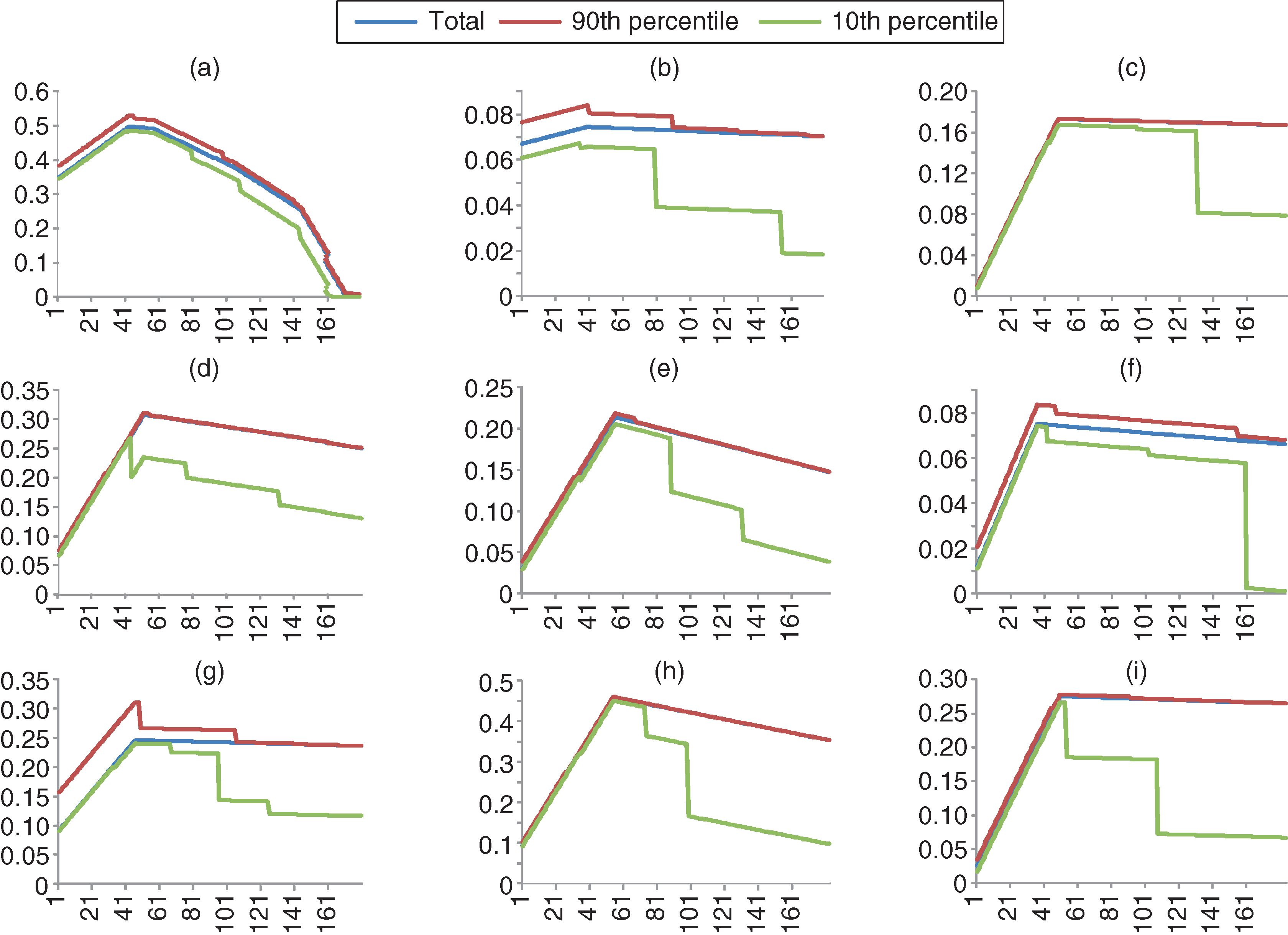
Figure 2: Impulse response functions for the multivariate time-varying Bayesian panel VAR model. (a) Total electricity. (b) Electricity from coal. (c) Electricity from nuclear. (d) Electricity from natural gas. (e) Electricity from oil. (f) Electricity from hydro. (g) Electricity from biomass. (h) Electricity from solar. (i) Electricity from wind. Horizontal axis shows time in months.

We now turn our attention to the examination of IRFs drawn from the multivariate model (Figure 2). More specifically, the figure presents the new IRFs of GDP per capita growth to both aggregate and decomposed electricity supply shocks. It shows the typical speed of response to fluctuations in electricity generation and underscores the point that the responses of GDP growth may differ substantially, depending on the length of the electricity supply shocks.

Parts (a)–(c) of Figure 2 show the IRFs of the GDP growth to the transmission of electricity supply shocks (total, coal and nuclear). Specifically, the effect on US macroeconomic performance of a one standard deviation shock of the total electricity generation when all the covariates enter the model is positive and significant only in the short run (three years after the initial shock). The figure reveals that a subsequent increase in electricity generation, all else being equal, would cause a continuous downward trend in GDP growth within the next month, which stabilizes thereafter. Lastly, the cumulative peak response of GDP growth to total electricity innovations occurs three years after the initial shock and is estimated to be approximately 5%, which is higher than the equivalent response of the bivariate model (approximately 3.5%). Moreover, as can easily be observed from Figure 2, the IRFs show similar behavior across all forms of electricity supply (as well as across all three distributions), confirming the important role of electricity (regardless of the source of energy that generates it) for economic growth across the US states.

Finally, if we try to compare the IRFs between the two (bivariate and multivariate) models, some interesting results emerge. First, the response of GDP growth per capita to electricity supply shocks is steeper in the multivariate model than the bivariate model, since the relevant peak response in the short run is higher in the former than the latter. However, both models exhibit a decreasing trend for nearly three years, on average, after the shock, stabilizing thereafter. This finding reveals the absence of a sluggish adjustment mechanism, which may reflect weak competition and significant market power by the incumbents in the electricity industry. Moreover, any electricity shock is short lived in both models. Specifically, the rate of response of GDP growth per capita to electricity supply shocks indicates that a market power effect prevails in the electricity industry.

7 Conclusions and policy implications

The goal of this paper was to investigate the relationship and the possible spillovers between electricity supply shocks and macroeconomic performance in the United States. The analysis used monthly seasonally adjusted regional data across forty-eight US states and combined a novel identification strategy for electricity supply shocks based on inequality constraints with the estimation of a time-varying Bayesian VAR model. The main novelty of this paper was that, for the first time (to the authors’ knowledge) in the empirical literature, it used a TVBPVAR model accounting for the decomposition of electricity supply per fuel mixture and linking its possible interactions with US macroeconomic conditions.

The empirical findings clearly illustrate that the US macroeconomic performance improved following a positive electricity supply shock (regardless of the energy source it originated). These findings survived a robustness check based on a multivariate model that identified several economic drivers for growth. These results could be important for policy makers, academic researchers and government officials. More specifically, they call for the need to strengthen the effectiveness of energy-generating agencies by ensuring systematic replacements of worn-out equipment and necessary tools to drastically reduce power losses. Any electricity outages are expected to have spillovers from the distorted macroeconomic performance that affect both domestic and global welfare.

US energy policy makers should design and implement efficient electricity conservation policies without adversely affecting economic growth. Such policies aim at reducing the wastage of electricity, such as demand-side management and efficiency improvement measures. Therefore, to ensure the security of supply to meet the demand of electricity, they need to primarily emphasize alternative sources of electricity, such as renewables, which were also shown to exert a positive impact on economic growth. The overall findings validate that electricity supply stimulates economic growth across US states. Intuitively, improvements in electricity supply are a necessity for the enhancement of the economy. Hence, policy makers should put in place any necessary policies that could restructure the electricity supply industry.

Declaration of interest

The authors report no conflicts of interest. The authors alone are responsible for the content and writing of the paper.

References

Alesina, A., and Roubini, N. (1997). Political Business Cycles and the Macroeconomy. MIT Press, Cambridge, MA (https://doi.org/10.7551/mitpress/5437.001.0001).
Allcott, H., Collard-Wexler, A., and O’Connell, S. D. (2016). How do electricity shortages affect industry? Evidence from India. American Economic Review 106(3), 587–624.
Andersen, T. B., and Dalgaard, C. J. (2013). Power outages and economic growth in Africa. Energy Economics 38, 19–23 (https://doi.org/10.1016/j.eneco.2013.02.016).
Assenmacher-Wesche, K., and Gerlach, S. (2010). Financial structure and the impact of monetary policy on property prices. Working Paper, Swiss National Bank.
Azariadis, C., and Drazen, A. (1990). Threshold externalities in economic development. Quarterly Journal of Economics 105(2), 501–526 (https://doi.org/10.2307/2937797).
Balducci, P. J., Roop, J. M., Schienbein, L. A., Desteese, J. G., and Weimar, M. R. (2002). Electrical power interruption cost estimates for individual industries, sectors and US economy. Technical Report PNNL-13797, Pacific Northwest National Laboratory, US Department of Energy (https://doi.org/10.2172/926127).
Barro, R. J. (1990). Government spending in a simple model of endogenous growth. Journal of Political Economy 98(5), 103–125 (https://doi.org/10.1086/261726).
Barsky, R. B., and Kilian, L. (2002). Do we really know that oil caused the Great Stagflation? A monetary alternative. NBER Macroeconomics Annual 16, 137–198 (https://doi.org/10.1086/654439).
Bildirici, M. E., Bakirtas, T., and Kayikci, F. (2012). Economic growth and electricity consumption: auto regressive distributed lag analysis. Journal of Energy in Southern Africa 23(4), 29–45 (https://doi.org/10.17159/2413-3051/2012/v23i4a3176).
Bucci, A., and La Torre, D. (2007). Population and economic growth with human and physical capital investments. Departmental Working Paper 2007-45, Department of Economics, University of Milan.
Calza, A., Monacelli, T., and Stracca, L. (2013). Housing finance and monetary policy. Journal of the European Economic Association 11, 101–122 (https://doi.org/10.1111/j.1542-4774.2012.01095.x).
Canova, F., and Ciccarelli, M. (2013). Panel vector autoregressive models: a survey. Working Paper 1507, European Central Bank, Frankfurt. URL: http://www.ecb.europa.eu/pub/pdf/scpwps/ecbwp1507.pdf.
Cheng, Y. S., Wong, W. K., and Woo. C. K. (2013). How much have electricity shortages hampered China’s GDP growth? Energy Policy 55, 369–373 (https://doi.org/10.1016/j.enpol.2012.12.015).
Cogley, T., and Sargent, T. (2005). Drift and volatilities: monetary policies and outcomes in the post WWII US. Review of Economic Dynamics 8(2), 262–302 (https://doi.org/10.1016/j.red.2004.10.009).
Dawson, D. J., and Tiffin, R. (1998). Is there a long-run relationship between population growth and living standards? The case of India. Journal of Development Studies 34(5), 149–156 (https://doi.org/10.1080/00220389808422540).
de Nooij, M., Koopmans, C., and Bijvoet, C. (2007). The value of supply security: the costs of power interruptions – economic input for damage reduction and investment in networks. Energy Economics 29(2), 277–295 (https://doi.org/10.1016/j.eneco.2006.05.022).
Faust, J., and Irons, J. (1999). Money, politics and the post-war business cycle. Journal of Monetary Economics 43(1), 61–89 (https://doi.org/10.1016/S0304-3932(98)00046-4).
Frankel, J., and Romer, D. 1999. Does trade cause growth? American Economic Review 89(3), 379–399 (https://doi.org/10.1257/aer.89.3.379).
Giulietti, M., Otero, J., and Waterson, M. (2010). Pricing behaviour under competition in the UK electricity supply industry. Oxford Economic Papers 62(3), 478–503 (https://doi.org/10.1093/oep/gpp029).
Gómez, M. A. (2007). Fiscal policy, congestion, and endogenous growth. Journal of Public Economic Theory 10(4), 595–622 (https://doi.org/10.1111/j.1467-9779.2008.00378.x).
Grasso, M. (2010). Time-varying parameters Bayesian forecasting of electricity demand: the Italian case. Working Paper 36, IEFE, Bocconi University, Milan (https://doi.org/10.2139/ssrn.1648786).
Hamilton, J. D. (2003). What is an oil shock? Journal of Econometrics 113(2), 363–398 (https://doi.org/10.1016/S0304-4076(02)00207-5).
Hong, Z., and Lian, H. (2012). Time-varying coefficient estimation in differential equation models with noisy time-varying covariates. Journal of Multivariate Analysis 103(1), 58–67 (https://doi.org/10.1016/j.jmva.2011.06.007).
Hunt, A., Collard-Wexler, A. C., and O’Connell, S. D. (2016). How do electricity shortages affect industry? Evidence from India. American Economic Review 106(3), 587–624 (https://doi.org/10.1257/aer.20140389).
Hurn, S., Silvennoinen, A., and Teräsvirta, T. (2016). A smooth transition logit model of the effects of deregulation in the electricity market. Journal of Applied Econometrics 31(4), 707–733 (https://doi.org/10.1002/jae.2452).
International Energy Agency (2019). Energy policies of IEA countries: the United States 2019 review. Report, IEA, Paris. URL: https://bit.ly/34bn1ac.
Irwin, D. A., and Terviö, M. (2002). Does trade raise income? Evidence from the twentieth century. Journal of International Economics 58(1), 1–18 (https://doi.org/10.1016/S0022-1996(01)00164-7).
Jakovac, P., and Vlahinić Lenz, N. (2016). Energy and economy in the Republic of Croatia: macroeconomic effects of electricity generation and consumption. Monograph, University of Rijeka (in Croatian). URL: https://bit.ly/3cnMGA8.
Joskow, P. (2001). California’s electricity crisis. Oxford Review of Economic Policy 17(3), 365–388 (https://doi.org/10.1093/oxrep/17.3.365).
Joskow, P., and Kohn, E. (2002). A quantitative analysis of pricing behavior in California’s wholesale electricity market during summer 2000. Energy Journal 23(4), 1–35 (https://doi.org/10.5547/ISSN0195-6574-EJ-Vol23-No4-1).
Karras, G. (2008). Trade openness and economic growth: can we estimate the precise effect? Applied Econometrics and International Development 3(1), 7–25. URL: http://www.usc.gal/economet/reviews/aeid311.pdf.
Kilian, L. (2008a). Exogenous oil supply shocks: how big are they and how much do they matter for the US economy? Review of Economics and Statistics 90(2), 216–240 (https://doi.org/10.1162/rest.90.2.216).
Kilian, L. (2008b). A comparison of the effects of exogenous oil supply shocks on output and inflation in the G7 countries. Journal of the European Economic Association 6(1), 78–121 (https://doi.org/10.1162/JEEA.2008.6.1.78).
Kilian, L. (2009a). Comment on “Causes and consequences of the oil shock of 2007–08” by James D. Hamilton. Brookings Papers on Economic Activity 2009(1), 267–278 (https://doi.org/10.1353/eca.0.0047).
Kilian, L. (2009b). Not all oil price shocks are alike: disentangling demand and supply shocks in the crude oil market. American Economic Review 99(3), 1053–1069 (https://doi.org/10.1257/aer.99.3.1053).
Kilian, L., and Murphy, D. (2013). The role of inventories and speculative trading in the global market for crude oil. Journal of Applied Econometrics 29(3), 454–478 (https://doi.org/10.1002/jae.2322).
Klenow, P., and Rodríguez-Clare, A. (1997). Economic growth, a review essay. Journal of Monetary Economics 40(3), 597–617 (https://doi.org/10.1016/S0304-3932(97)00050-0).
Kneller, R., Bleaney, M. F., and Gemmell, N. (1999). Fiscal policy and growth: evidence from OECD countries. Journal of Public Economics 74(2), 171–190 (https://doi.org/10.1016/S0047-2727(99)00022-5).
Levine, P., Stern, J., and Trillas, F. (2005). Utility price regulation and time inconsistency: comparisons with monetary policy. Oxford Economic Papers 57(3), 447–478 (https://doi.org/10.1093/oep/gpi021).
Liu, S., You, J., and Heng, L. (2017). Estimation and model identification of longitudinal data time-varying nonparametric models. Journal of Multivariate Analysis 156, 116–136 (https://doi.org/10.1016/j.jmva.2017.02.003).
Lorde, T., Waithe, K., and Francis, B. (2010). The importance of electrical energy for economic growth in Barbados. Energy Economics 32(6), 1411–1420 (https://doi.org/10.1016/j.eneco.2010.05.011).
Lucas, R. E., Jr. (1988). On the mechanics of economic development. Journal of Monetary Economics 22(1), 3–42 (https://doi.org/10.1016/0304-3932(88)90168-7).
Mamatzakis, E., Kalyvas, A. N., and Piesse, J. (2013). Does regulation in credit, labour and business matter for bank performance in the EU-10 economies? International Journal of the Economics of Business 20(3), 341–385 (https://doi.org/10.1080/13571516.2013.835981).
Mertens, K. (2008). Deposit rate ceilings and monetary transmission in the US. Journal of Monetary Economics 55(7), 1290–1302 (https://doi.org/10.1016/j.jmoneco.2008.08.007).
Narayan, P. K., Narayan, S., and Popp, S. (2010). Does electricity consumption panel Granger cause GDP? A new global evidence. Applied Energy 87(10), 3294–3298 (https://doi.org/10.1016/j.apenergy.2010.03.021).
Olivei, G., and Tenreyro, S. (2007). The timing of monetary policy shocks. American Economic Review 97(3), 636–663 (https://doi.org/10.1257/aer.97.3.636).
Olivei, G., and Tenreyro, S. (2010). Wage-setting patterns and monetary policy: international evidence. Journal of Monetary Economics 57(7), 785–802 (https://doi.org/10.1016/j.jmoneco.2010.08.003).
Pede, V. O. (2013). Diversity and regional economic growth: evidence from US counties. Journal of Economic Development 38(3), 111–127 (https://doi.org/10.35866/caujed.2013.38.3.005).
Pereira, M. C., and Lopes, A. S. (2010). Time-varying fiscal policy in the US. Working Paper 21, Economics and Research Department, Bank of Portugal. URL: http://www.bportugal.pt/sites/default/files/anexos/papers/wp201021.pdf.
Pesaran, M. H. (2004). General diagnostic tests for cross section dependence in panels. Working Paper 435, Cambridge Working Papers in Economics (https://doi.org/10.17863/CAM.5113)
Pesaran, M. H. (2007). A simple panel unit root test in the presence of cross-section dependence. Journal of Applied Econometrics 22(2), 265–312 (https://doi.org/10.1002/jae.951).
Polemis, M. (2016). New evidence on the impact of structural reforms on electricity sector performance. Energy Policy 92, 420–431 (https://doi.org/10.1016/j.enpol.2016.02.032).
Poudineh, R., and Jamasb, T. (2017). Electricity supply interruptions: sectoral interdependencies and the cost of energy not served for the Scottish economy. Energy Journal 38(1), 51–76 (https://doi.org/10.5547/01956574.38.1.rpou).
Ramey, V. A., and Vine, D. (2011). Oil, automobiles, and the US economy: how much have things really changed? NBER Macroeconomics Annual 25, 333–367 (https://doi.org/10.1086/657541).
Rebelo, S. (1991). Long-run policy analysis and long-run growth. Journal of Political Economy 99(3), 500–512 (https://doi.org/10.1086/261764).
Reed, R. W. (2009). The determinants of US state economic growth: a less extreme bounds analysis. Economic Inquiry 47(4), 685–700 (https://doi.org/10.1111/j.1465-7295.2008.00127.x).
Reichl, J., Schmidthaler, M., and Schneider, F. (2013). The value of supply security: the costs of power outages to Austrian households, firms and the public sector. Energy Economics 36, 256–261 (https://doi.org/10.1016/j.eneco.2012.08.044).
Romer, P. M. (1986). Increasing returns and long-run growth. Journal of Political Economy 94(5), 1002–1037 (https://doi.org/10.1086/261420).
Santa-Clara, P., and Valkanov, R. (2003). The presidential puzzle: political cycles and the stock market. Journal of Finance 58(5), 1841–1872 (https://doi.org/10.1111/1540-6261.00590).
Solarin, S. A., and Shahbaz, M. (2013). Trivariate causality between economic growth, urbanisation and electricity consumption in Angola: cointegration and causality analysis. Energy Policy 60, 876–884 (https://doi.org/10.1016/j.enpol.2013.05.058).
Szirmai, A. (2012). Industrialisation as an engine of growth in developing countries, 1950–2005. Structural Change and Economic Dynamics 23(4), 406–420 (https://doi.org/10.1016/j.strueco.2011.01.005).
Tarr, D. (2012). Impact of services liberalization on industry productivity, exports and development: six empirical studies in the transition countries. Policy Research Working Paper 6023, World Bank, Washington, DC (https://doi.org/10.1596/1813-9450-6023).
Thornton, J. (2001). Population growth and economic growth: long-run evidence from Latin America. Southern Economic Journal 68(2), 464–468 (https://doi.org/10.2307/1061606).
Toba, N. (2007). Welfare impacts of electricity generation sector reform in the Philippines. Energy Policy 35(12), 6145–6162 (https://doi.org/10.1016/j.enpol.2007.07.018).
Turok, I., and McGranahan, G. (2013). Urbanization and economic growth: the arguments and evidence for Africa and Asia. Environment and Urbanization 25(2), 465–482 (https://doi.org/10.1177/0956247813490908).
Ulku, H. (2004). R&D, innovation, and economic growth: an empirical analysis. Working Paper 185-04, International Monetary Fund, Washington, DC (https://doi.org/10.5089/9781451859447.001).
US Department of Energy (2015). United States electricity industry primer. Report DOE/OE-0017, Office of Electricity Delivery and Energy Reliability, US Department of Energy, Washington, DC. URL: http://www.energy.gov/sites/prod/files/2015/12/f28/united-states-electricity-industry-primer.pdf.
Weber, J. G., Wall, C., Brown, J., and Hertz, T. (2015). Crop prices, agricultural revenues, and the rural economy. Applied Economic Perspectives and Policy 37(3), 459–476 (https://doi.org/10.1093/aepp/ppu040).
Wieladek, T. (2016). The varying coefficient Bayesian panel VAR model. Staff Working Paper 578, Bank of England, London (https://doi.org/10.2139/ssrn.2713856).
Young, A. (1991). Learning by doing and the dynamic effects of international trade. Quarterly Journal of Economics 106(2), 369–406 (https://doi.org/10.2307/2937942).
Young, A. (1995). The tyranny of numbers: confronting the statistical realities of the East Asian growth experience. Quarterly Journal of Economics 110(3), 641–680 (https://doi.org/10.2307/2946695).
Zagler, M., and Dürnecker, G. (2003). Fiscal policy and economic growth. Journal of Economic Surveys 17(3), 397–418 (https://doi.org/10.1111/1467-6419.00199).

[bib.bib2] Alesina, A., and Roubini, N. (1997). Political Business Cycles and the Macroeconomy. MIT Press, Cambridge, MA (https://doi.org/10.7551/mitpress/5437.001.0001).

[bib.bib4] Allcott, H., Collard-Wexler, A., and O’Connell, S. D. (2016). How do electricity shortages affect industry? Evidence from India. American Economic Review 106(3), 587–624.

[bib.bib6] Andersen, T. B., and Dalgaard, C. J. (2013). Power outages and economic growth in Africa. Energy Economics 38, 19–23 (https://doi.org/10.1016/j.eneco.2013.02.016).

[bib.bib8] Assenmacher-Wesche, K., and Gerlach, S. (2010). Financial structure and the impact of monetary policy on property prices. Working Paper, Swiss National Bank.

[bib.bib10] Azariadis, C., and Drazen, A. (1990). Threshold externalities in economic development. Quarterly Journal of Economics 105(2), 501–526 (https://doi.org/10.2307/2937797).

[bib.bib12] Balducci, P. J., Roop, J. M., Schienbein, L. A., Desteese, J. G., and Weimar, M. R. (2002). Electrical power interruption cost estimates for individual industries, sectors and US economy. Technical Report PNNL-13797, Pacific Northwest National Laboratory, US Department of Energy (https://doi.org/10.2172/926127).

[bib.bib14] Barro, R. J. (1990). Government spending in a simple model of endogenous growth. Journal of Political Economy 98(5), 103–125 (https://doi.org/10.1086/261726).

[bib.bib16] Barsky, R. B., and Kilian, L. (2002). Do we really know that oil caused the Great Stagflation? A monetary alternative. NBER Macroeconomics Annual 16, 137–198 (https://doi.org/10.1086/654439).

[bib.bib18] Bildirici, M. E., Bakirtas, T., and Kayikci, F. (2012). Economic growth and electricity consumption: auto regressive distributed lag analysis. Journal of Energy in Southern Africa 23(4), 29–45 (https://doi.org/10.17159/2413-3051/2012/v23i4a3176).

[bib.bib20] Bucci, A., and La Torre, D. (2007). Population and economic growth with human and physical capital investments. Departmental Working Paper 2007-45, Department of Economics, University of Milan.

[bib.bib22] Calza, A., Monacelli, T., and Stracca, L. (2013). Housing finance and monetary policy. Journal of the European Economic Association 11, 101–122 (https://doi.org/10.1111/j.1542-4774.2012.01095.x).

[bib.bib24] Canova, F., and Ciccarelli, M. (2013). Panel vector autoregressive models: a survey. Working Paper 1507, European Central Bank, Frankfurt. URL: http://www.ecb.europa.eu/pub/pdf/scpwps/ecbwp1507.pdf.

[bib.bib26] Cheng, Y. S., Wong, W. K., and Woo. C. K. (2013). How much have electricity shortages hampered China’s GDP growth? Energy Policy 55, 369–373 (https://doi.org/10.1016/j.enpol.2012.12.015).

[bib.bib28] Cogley, T., and Sargent, T. (2005). Drift and volatilities: monetary policies and outcomes in the post WWII US. Review of Economic Dynamics 8(2), 262–302 (https://doi.org/10.1016/j.red.2004.10.009).

[bib.bib30] Dawson, D. J., and Tiffin, R. (1998). Is there a long-run relationship between population growth and living standards? The case of India. Journal of Development Studies 34(5), 149–156 (https://doi.org/10.1080/00220389808422540).

[bib.bib32] de Nooij, M., Koopmans, C., and Bijvoet, C. (2007). The value of supply security: the costs of power interruptions – economic input for damage reduction and investment in networks. Energy Economics 29(2), 277–295 (https://doi.org/10.1016/j.eneco.2006.05.022).

[bib.bib34] Faust, J., and Irons, J. (1999). Money, politics and the post-war business cycle. Journal of Monetary Economics 43(1), 61–89 (https://doi.org/10.1016/S0304-3932(98)00046-4).

[bib.bib36] Frankel, J., and Romer, D. 1999. Does trade cause growth? American Economic Review 89(3), 379–399 (https://doi.org/10.1257/aer.89.3.379).

[bib.bib38] Giulietti, M., Otero, J., and Waterson, M. (2010). Pricing behaviour under competition in the UK electricity supply industry. Oxford Economic Papers 62(3), 478–503 (https://doi.org/10.1093/oep/gpp029).

[bib.bib40] Gómez, M. A. (2007). Fiscal policy, congestion, and endogenous growth. Journal of Public Economic Theory 10(4), 595–622 (https://doi.org/10.1111/j.1467-9779.2008.00378.x).

[bib.bib42] Grasso, M. (2010). Time-varying parameters Bayesian forecasting of electricity demand: the Italian case. Working Paper 36, IEFE, Bocconi University, Milan (https://doi.org/10.2139/ssrn.1648786).

[bib.bib44] Hamilton, J. D. (2003). What is an oil shock? Journal of Econometrics 113(2), 363–398 (https://doi.org/10.1016/S0304-4076(02)00207-5).

[bib.bib46] Hong, Z., and Lian, H. (2012). Time-varying coefficient estimation in differential equation models with noisy time-varying covariates. Journal of Multivariate Analysis 103(1), 58–67 (https://doi.org/10.1016/j.jmva.2011.06.007).

[bib.bib48] Hunt, A., Collard-Wexler, A. C., and O’Connell, S. D. (2016). How do electricity shortages affect industry? Evidence from India. American Economic Review 106(3), 587–624 (https://doi.org/10.1257/aer.20140389).

[bib.bib50] Hurn, S., Silvennoinen, A., and Teräsvirta, T. (2016). A smooth transition logit model of the effects of deregulation in the electricity market. Journal of Applied Econometrics 31(4), 707–733 (https://doi.org/10.1002/jae.2452).

[bib.bib52] International Energy Agency (2019). Energy policies of IEA countries: the United States 2019 review. Report, IEA, Paris. URL: https://bit.ly/34bn1ac.

[bib.bib54] Irwin, D. A., and Terviö, M. (2002). Does trade raise income? Evidence from the twentieth century. Journal of International Economics 58(1), 1–18 (https://doi.org/10.1016/S0022-1996(01)00164-7).

[bib.bib56] Jakovac, P., and Vlahinić Lenz, N. (2016). Energy and economy in the Republic of Croatia: macroeconomic effects of electricity generation and consumption. Monograph, University of Rijeka (in Croatian). URL: https://bit.ly/3cnMGA8.

[bib.bib58] Joskow, P. (2001). California’s electricity crisis. Oxford Review of Economic Policy 17(3), 365–388 (https://doi.org/10.1093/oxrep/17.3.365).

[bib.bib60] Joskow, P., and Kohn, E. (2002). A quantitative analysis of pricing behavior in California’s wholesale electricity market during summer 2000. Energy Journal 23(4), 1–35 (https://doi.org/10.5547/ISSN0195-6574-EJ-Vol23-No4-1).

[bib.bib62] Karras, G. (2008). Trade openness and economic growth: can we estimate the precise effect? Applied Econometrics and International Development 3(1), 7–25. URL: http://www.usc.gal/economet/reviews/aeid311.pdf.

[bib.bib64] Kilian, L. (2008a). Exogenous oil supply shocks: how big are they and how much do they matter for the US economy? Review of Economics and Statistics 90(2), 216–240 (https://doi.org/10.1162/rest.90.2.216).

[bib.bib66] Kilian, L. (2008b). A comparison of the effects of exogenous oil supply shocks on output and inflation in the G7 countries. Journal of the European Economic Association 6(1), 78–121 (https://doi.org/10.1162/JEEA.2008.6.1.78).

[bib.bib68] Kilian, L. (2009a). Comment on “Causes and consequences of the oil shock of 2007–08” by James D. Hamilton. Brookings Papers on Economic Activity 2009(1), 267–278 (https://doi.org/10.1353/eca.0.0047).

[bib.bib70] Kilian, L. (2009b). Not all oil price shocks are alike: disentangling demand and supply shocks in the crude oil market. American Economic Review 99(3), 1053–1069 (https://doi.org/10.1257/aer.99.3.1053).

[bib.bib72] Kilian, L., and Murphy, D. (2013). The role of inventories and speculative trading in the global market for crude oil. Journal of Applied Econometrics 29(3), 454–478 (https://doi.org/10.1002/jae.2322).

[bib.bib74] Klenow, P., and Rodríguez-Clare, A. (1997). Economic growth, a review essay. Journal of Monetary Economics 40(3), 597–617 (https://doi.org/10.1016/S0304-3932(97)00050-0).

[bib.bib76] Kneller, R., Bleaney, M. F., and Gemmell, N. (1999). Fiscal policy and growth: evidence from OECD countries. Journal of Public Economics 74(2), 171–190 (https://doi.org/10.1016/S0047-2727(99)00022-5).

[bib.bib78] Levine, P., Stern, J., and Trillas, F. (2005). Utility price regulation and time inconsistency: comparisons with monetary policy. Oxford Economic Papers 57(3), 447–478 (https://doi.org/10.1093/oep/gpi021).

[bib.bib80] Liu, S., You, J., and Heng, L. (2017). Estimation and model identification of longitudinal data time-varying nonparametric models. Journal of Multivariate Analysis 156, 116–136 (https://doi.org/10.1016/j.jmva.2017.02.003).

[bib.bib82] Lorde, T., Waithe, K., and Francis, B. (2010). The importance of electrical energy for economic growth in Barbados. Energy Economics 32(6), 1411–1420 (https://doi.org/10.1016/j.eneco.2010.05.011).

[bib.bib84] Lucas, R. E., Jr. (1988). On the mechanics of economic development. Journal of Monetary Economics 22(1), 3–42 (https://doi.org/10.1016/0304-3932(88)90168-7).

[bib.bib86] Mamatzakis, E., Kalyvas, A. N., and Piesse, J. (2013). Does regulation in credit, labour and business matter for bank performance in the EU-10 economies? International Journal of the Economics of Business 20(3), 341–385 (https://doi.org/10.1080/13571516.2013.835981).

[bib.bib88] Mertens, K. (2008). Deposit rate ceilings and monetary transmission in the US. Journal of Monetary Economics 55(7), 1290–1302 (https://doi.org/10.1016/j.jmoneco.2008.08.007).

[bib.bib90] Narayan, P. K., Narayan, S., and Popp, S. (2010). Does electricity consumption panel Granger cause GDP? A new global evidence. Applied Energy 87(10), 3294–3298 (https://doi.org/10.1016/j.apenergy.2010.03.021).

[bib.bib92] Olivei, G., and Tenreyro, S. (2007). The timing of monetary policy shocks. American Economic Review 97(3), 636–663 (https://doi.org/10.1257/aer.97.3.636).

[bib.bib94] Olivei, G., and Tenreyro, S. (2010). Wage-setting patterns and monetary policy: international evidence. Journal of Monetary Economics 57(7), 785–802 (https://doi.org/10.1016/j.jmoneco.2010.08.003).

[bib.bib96] Pede, V. O. (2013). Diversity and regional economic growth: evidence from US counties. Journal of Economic Development 38(3), 111–127 (https://doi.org/10.35866/caujed.2013.38.3.005).

[bib.bib98] Pereira, M. C., and Lopes, A. S. (2010). Time-varying fiscal policy in the US. Working Paper 21, Economics and Research Department, Bank of Portugal. URL: http://www.bportugal.pt/sites/default/files/anexos/papers/wp201021.pdf.

[bib.bib100] Pesaran, M. H. (2004). General diagnostic tests for cross section dependence in panels. Working Paper 435, Cambridge Working Papers in Economics (https://doi.org/10.17863/CAM.5113)

[bib.bib102] Pesaran, M. H. (2007). A simple panel unit root test in the presence of cross-section dependence. Journal of Applied Econometrics 22(2), 265–312 (https://doi.org/10.1002/jae.951).

[bib.bib104] Polemis, M. (2016). New evidence on the impact of structural reforms on electricity sector performance. Energy Policy 92, 420–431 (https://doi.org/10.1016/j.enpol.2016.02.032).

[bib.bib106] Poudineh, R., and Jamasb, T. (2017). Electricity supply interruptions: sectoral interdependencies and the cost of energy not served for the Scottish economy. Energy Journal 38(1), 51–76 (https://doi.org/10.5547/01956574.38.1.rpou).

[bib.bib108] Ramey, V. A., and Vine, D. (2011). Oil, automobiles, and the US economy: how much have things really changed? NBER Macroeconomics Annual 25, 333–367 (https://doi.org/10.1086/657541).

[bib.bib110] Rebelo, S. (1991). Long-run policy analysis and long-run growth. Journal of Political Economy 99(3), 500–512 (https://doi.org/10.1086/261764).

[bib.bib112] Reed, R. W. (2009). The determinants of US state economic growth: a less extreme bounds analysis. Economic Inquiry 47(4), 685–700 (https://doi.org/10.1111/j.1465-7295.2008.00127.x).

[bib.bib114] Reichl, J., Schmidthaler, M., and Schneider, F. (2013). The value of supply security: the costs of power outages to Austrian households, firms and the public sector. Energy Economics 36, 256–261 (https://doi.org/10.1016/j.eneco.2012.08.044).

[bib.bib116] Romer, P. M. (1986). Increasing returns and long-run growth. Journal of Political Economy 94(5), 1002–1037 (https://doi.org/10.1086/261420).

[bib.bib118] Santa-Clara, P., and Valkanov, R. (2003). The presidential puzzle: political cycles and the stock market. Journal of Finance 58(5), 1841–1872 (https://doi.org/10.1111/1540-6261.00590).

[bib.bib120] Solarin, S. A., and Shahbaz, M. (2013). Trivariate causality between economic growth, urbanisation and electricity consumption in Angola: cointegration and causality analysis. Energy Policy 60, 876–884 (https://doi.org/10.1016/j.enpol.2013.05.058).

[bib.bib122] Szirmai, A. (2012). Industrialisation as an engine of growth in developing countries, 1950–2005. Structural Change and Economic Dynamics 23(4), 406–420 (https://doi.org/10.1016/j.strueco.2011.01.005).

[bib.bib124] Tarr, D. (2012). Impact of services liberalization on industry productivity, exports and development: six empirical studies in the transition countries. Policy Research Working Paper 6023, World Bank, Washington, DC (https://doi.org/10.1596/1813-9450-6023).

[bib.bib126] Thornton, J. (2001). Population growth and economic growth: long-run evidence from Latin America. Southern Economic Journal 68(2), 464–468 (https://doi.org/10.2307/1061606).

[bib.bib128] Toba, N. (2007). Welfare impacts of electricity generation sector reform in the Philippines. Energy Policy 35(12), 6145–6162 (https://doi.org/10.1016/j.enpol.2007.07.018).

[bib.bib130] Turok, I., and McGranahan, G. (2013). Urbanization and economic growth: the arguments and evidence for Africa and Asia. Environment and Urbanization 25(2), 465–482 (https://doi.org/10.1177/0956247813490908).

[bib.bib132] Ulku, H. (2004). R&D, innovation, and economic growth: an empirical analysis. Working Paper 185-04, International Monetary Fund, Washington, DC (https://doi.org/10.5089/9781451859447.001).

[bib.bib134] US Department of Energy (2015). United States electricity industry primer. Report DOE/OE-0017, Office of Electricity Delivery and Energy Reliability, US Department of Energy, Washington, DC. URL: http://www.energy.gov/sites/prod/files/2015/12/f28/united-states-electricity-industry-primer.pdf.

[bib.bib136] Weber, J. G., Wall, C., Brown, J., and Hertz, T. (2015). Crop prices, agricultural revenues, and the rural economy. Applied Economic Perspectives and Policy 37(3), 459–476 (https://doi.org/10.1093/aepp/ppu040).

[bib.bib138] Wieladek, T. (2016). The varying coefficient Bayesian panel VAR model. Staff Working Paper 578, Bank of England, London (https://doi.org/10.2139/ssrn.2713856).

[bib.bib140] Young, A. (1991). Learning by doing and the dynamic effects of international trade. Quarterly Journal of Economics 106(2), 369–406 (https://doi.org/10.2307/2937942).

[bib.bib142] Young, A. (1995). The tyranny of numbers: confronting the statistical realities of the East Asian growth experience. Quarterly Journal of Economics 110(3), 641–680 (https://doi.org/10.2307/2946695).

[bib.bib144] Zagler, M., and Dürnecker, G. (2003). Fiscal policy and economic growth. Journal of Economic Surveys 17(3), 397–418 (https://doi.org/10.1111/1467-6419.00199).

Journal of Energy Markets

Decomposing supply shocks in the US electricity industry: evidence from a time-varying Bayesian panel vector autoregression model

Nicholas Apergis and Michael Polemis

Need to know

Abstract

Introduction