Journal of Network Theory in Finance
ISSN:
2055-7795 (print)
2055-7809 (online)
Editor-in-chief: Ron Berndsen

Relation between regional uncertainty spillovers in the global banking system
Need to know
- We add exponential weighting to the method of Diebold and Yilmaz.
- We construct time series of uncertainty for three regional banking systems.
- We find significant causal relations between uncertainty in the three regions.
Abstract
We report on time-varying network connectedness within three banking systems: North America (NA), the European Union (EU) and Southeast Asia (ASEAN). Diebold and Yilmaz’s original method is improved by using exponentially weighted daily returns as well as ridge regularization on vector autoregression (VAR) and fore- cast error variance decomposition (FEVD). We compute the total network connectedness for each of the three banking systems, which quantifies regional uncertainty. Results over rolling windows of 300 days during the period from January 2005 to October 2015 reveal changing uncertainty patterns that are similar across regions, demonstrating common peaks associated with identifiable exogenous events. Lead– lag relationships among changes of total network connectedness of the three systems, quantified by transfer entropy, reveal that uncertainties in the three regional systems are significantly causally related, with the NA system having the largest influence on the EU and ASEAN.
Introduction
1 Introduction
Financial markets are increasingly becoming more interconnected (Moghadam and Vinals 2010), and shocks initially affecting one part of the system can quickly propagate to the rest of it. Therefore, understanding the patterns of distress propagation within financial markets is important to characterize systemic risk. After the global financial crisis of 2007–9, significant effort has been devoted to understanding the mechanics of distress propagation within banking systems. One strand of the literature has focused on modeling the processes through which contagion may occur in interbank networks (see, for example, Glasserman and Young (2016) and Caccioli et al (2018) for recent reviews). Another strand of the literature has focused on the quantification of systemic risk from market data (see Adrian and Brunnermeier 2016; Brownlees and Engle 2016). In particular, Diebold and Yilmaz (2009) proposed a method based on forecast error variance decomposition (FEVD) of estimating from market data networks of interdependencies between firms, and they used the connectedness of the estimated networks to quantify spillovers of uncertainty between variables.
In this paper, we use the methodology of the aforementioned work by Diebold and Yilmaz (2009) to estimate the time evolution of connectedness in three regional banking systems: North America (NA), the European Union (EU) and Southeast Asia (ASEAN). Through VAR and FEVD, we compute the pairwise connectedness between pairs of banks in each region, and we aggregate such pairwise connectedness to compute a measure of total connectedness for the region.
The time-varying total connectedness computed for each banking system, from a 300-day rolling window during the period from January 2005 to October 2015, indicates temporal changes of systemic risk, with peaks during major crisis events and troughs during normal periods. Analogous results have been observed in other financial systems and different regions (Diebold and Yilmaz 2009, 2012, 2014; Chau and Deesomsak 2014; Alter and Beyer 2014; Fengler and Gisler 2015; Demirer et al 2018). It has to be stressed that, unlike Diebold and Yilmaz (2009), who view all financial institutions as belonging to one global system, here we group banks into three regional banking systems. In this way, we can perform a comparative analysis between the different regions, which allows us to highlight similarities and differences between them. Further, this allow us to quantify the existence of causal relations between different regions. Note that combining all the banks together could be somehow misleading, because the banks’ equities in the three banking systems trade in different stock markets that have significantly different trading hours.
The main results of our analysis are as follows. First, we note that the structure of the peaks in the three regional banking systems is very similar, with large peaks associated with significant, identifiable major events. Although the overall patterns are similar, we observe two important differences between the systems. The first is the fact that the overall scale of connectedness is different, with the NA banking system being more interconnected than that in the EU, which, in turn, is more interconnected than the ASEAN system. Second, we uncover the existence of lead–lagged relations between the different time series. To quantify this effect, we compute the transfer entropy between the time series associated with changes of connectedness in the different regions, and we uncover the existence of significant net information flows from NA to the EU, from NA to ASEAN, and from the EU to ASEAN. The robustness of our finding is tested using different measures for transfer entropy. In particular, we find consistent results for the net information flow both with a linear measure of transfer entropy (which corresponds to a Granger causality analysis) and with nonlinear measures of different parameters. We also retrieve similar causal relations for both one-day and five-day returns. To the best of our knowledge, this causality study between regional uncertainties is the first of its kind.
The rest of this paper is organized as follows. In Section 2, we present a literature review and place our paper in the context of previous works. In Section 3, we describe the used data, while Section 4 provides a brief description of our methodology. Section 5 illustrates and discusses the main results of the paper. We present our conclusions in Section 6.
2 Literature review
The literature on systemic risk and contagion in the banking network can be broadly classified into two categories. The first category comprises network models that aim to describe various causal mechanics of financial contagion, which can be calibrated with balance-sheet data (Furfine 2003; Degryse and Nguyen 2007; Upper and Worms 2004; Müller 2006; Cont et al 2010; Upper 2011; Birch and Aste 2014). The second category comprises econometric models that aim to identify spillover effects exclusively from market data, without making assumptions about the dynamics of distress propagation between banks (Adrian and Brunnermeier 2016; Brownlees and Engle 2016). Our paper is close to this second strand of the literature, as we try to understand whether market data carries information about the level of interconnectedness between banks and how exogenous shocks can be amplified by the endogenous dynamics of financial markets.
Network models of contagion go back to the seminal work of Allen and Gale (2000), who showed how the stability of the banking system is affected at equilibrium by the pattern of interconnections between banks, and to the work of Eisenberg and Noe (2001), who demonstrated how to consistently compute a clearing vector of payments in a network of interbank claims. The relation between the structure of an interbank network and its stability has also been extensively explored within the context of nonequilibrium network models (see, for example, Furfine 2003; Iori et al 2006; Nier et al 2007; Gai and Kapadia 2010; Cont et al 2010; Upper 2011; Battiston et al 2012; Fricke and Lux 2015; Bardoscia et al 2015, 2017; Kobayashi and Hasui 2014; Lenzu and Tedeschi 2012; Tedeschi et al 2001), showing in particular the existence of a tension between individual risk and systemic risk: what makes a bank individually less risky might in fact increase the risk of a systemic failure (Beale et al 2011). More recently, these analyses have been extended beyond interbank lending networks to the study of networks of overlapping portfolios (Huang et al 2013; Caccioli et al 2014; Corsi et al 2016). Although these models have been insightful with regard to understanding the dynamics of financial contagion, and in some cases they have been applied to real data (see Upper (2011) for a review of the existing literature), there are clear challenges to their applicability. First, there is a lack of reliable data on banks’ balance sheets, which makes it hard to calibrate models.11Admati et al (2013) report that banks tend to find ways to get around regulations in order to invest in mortgage-backed securities and derivatives via structured-investment vehicles, which are off-balance-sheet items. Such leeway being allowed by regulations creates regulatory boundaries, making it difficult for outsiders to know what banks actually report. Second, to obtain a reliable assessment of systemic risk one has to capture all relevant types of interconnections between banks, as the interaction between different contagion channels can significantly change the stability of the system (Caccioli et al 2015).
Here, we take the complementary approach of inferring interdependencies between banks from market data, which belongs to the second strand of literature mentioned above. The advantage of this approach with respect to network modeling is that market data is readily available, and different types of interconnections between banks have already been aggregated by the market. The drawback is that this approach does not provide an explanation of how stress propagates between banks, and it relies on the underlying assumption of market efficiency, which is not realistic (Shiller 2003). Nevertheless, one can assume that, although markets are not efficient, prices do reflect to some extent the aggregate information (or expectations) about the underlying assets. There have been several contributions to this strand of the literature. In particular, Dungey et al (2005) provide a summary of empirical models of contagion up to 2005. More recent empirical work includes Diebold and Yilmaz (2009, 2012, 2014), Caceres et al (2010), Billio et al (2012), Claeys and Vasicek (2014), Lucas et al (2014), Musmeci et al (2015) and Brownlees and Engle (2016). Of particular relevance for our paper is the work of Diebold and Yilmaz (2009, 2012, 2014), which influenced subsequent studies such as McMillan and Speight (2010), Bubák et al (2011), Fujiwara and Takahashi (2012), Klößner and Wagner (2014), Alter and Beyer (2014), Chau and Deesomsak (2014), Demirer et al (2018) and Fengler and Gisler (2015). This strand of contributions uses vector autoregression (VAR) and forecast error variance decomposition (FEVD) to quantify the unpredictability of each variable in the network. By using the VAR and FEVD methods, it is possible to disentangle the contribution to unpredictability due to endogenous interdependencies from that due to exogenous shocks. Following Diebold and Yilmaz, we will refer to this endogenous component in our paper as total network connectedness, which therefore quantifies the transmission of shocks from banks within the system.
3 Data
We collect daily stock prices from January 2005 to October 2015 of banks headquartered in NA (including the United States and Canada), the EU and ASEAN from the Compustat database. We select only financial institutions in the subindustry “Banks” (ie, large banks operating at the national level and having a GICS code of 40101010) and compute log returns from the daily closing prices for each bank. With the aforementioned criteria, our sample includes ten publicly listed banks in NA, sixty-six banks in the EU and thirty-nine banks in ASEAN that survived through the period January 2005–October 2015.
While we could analyze rolling windows in which the number of banks in operation varies from one window to the next, we find that being able to see the evolution of the systems’ total connectedness given a constant number of banks provides some baseline insight into how the same set of banks reacted to different economic and financial episodes over time. That being said, research that saw all surviving banks being accounted for in respective rolling windows would be an interesting avenue to explore. In such a case, the dimensions of the rolling windows would likely be much larger and estimation techniques such as sparsity modeling would be needed.
All banks in the NA banking system have their stocks traded in the New York Stock Exchange (NYSE), while the EU and ASEAN bank stocks mostly trade in their own national stock markets. Lists of banks in all three regions as well as their summary statistics are given in Tables 1–3.
| Daily | Daily | ||
|---|---|---|---|
| mean | volatility | ||
| Bank name | Country | return (%) | (%) |
| Canadian Imperial Bank (CIBC) | CAN | 0.01 | 1.82 |
| Bank of Montreal (BMO) | CAN | 0.01 | 1.69 |
| Royal Bank of Canada (RBC) | CAN | 0.03 | 1.73 |
| Toronto Dominion Bank (TD) | CAN | 0.03 | 1.65 |
| Bank of Nova Scotia (BNS) | CAN | 0.01 | 1.72 |
| Citigroup (CITI) | USA | 0.08 | 3.70 |
| Bank of America Corp (BAC) | USA | 0.04 | 3.51 |
| Wells Fargo & Co (WFC) | USA | 0.02 | 2.86 |
| JP Morgan Chase & Co (JPM) | USA | 0.02 | 2.64 |
| US Bancorp (USB) | USA | 0.01 | 2.32 |
| Market cap | Average | Volatility | ||
|---|---|---|---|---|
| Bank | Country | (USD billion) | return (%) | (%) |
| Bank Rakyat Indonesia | IDN | 20.43 | 0.07 | 2.56 |
| Bank Permata | IDN | 0.54 | 0.02 | 1.93 |
| Bank Danamon | IDN | 2.23 | 0.00 | 2.73 |
| Bank Maybank Indonesia | IDN | 0.79 | 0.00 | 2.67 |
| Bank Cimb Niaga | IDN | 1.07 | 0.02 | 2.51 |
| Panin Bank | IDN | 0.17 | 0.03 | 2.68 |
| Bank Negara Indonesia | IDN | 6.66 | 0.04 | 2.50 |
| Bank Central Asia | IDN | 23.21 | 0.08 | 2.06 |
| Bank Mandiri | IDN | 15.75 | 0.05 | 2.54 |
| Public Bank | MYS | 16.15 | 0.04 | 0.90 |
| Malayan Banking | MYS | 18.70 | 0.00 | 1.23 |
| RHB Capital | MYS | 3.73 | 0.03 | 1.58 |
| AMMB Holdings | MYS | 3.04 | 0.01 | 1.51 |
| AFFIN Holdings | MYS | 0.97 | 0.01 | 1.65 |
| Alliance Financial Group | MYS | 1.15 | 0.01 | 1.52 |
| BIMB Holdings | MYS | 1.35 | 0.03 | 2.13 |
| CIMB Group Holdings | MYS | 7.92 | 0.02 | 1.54 |
| Hong Leong Bank | MYS | 6.17 | 0.03 | 1.14 |
| Philippine National Bank | PHL | 1.20 | 0.03 | 2.39 |
| Bank of Philippine Islands | PHL | 6.97 | 0.03 | 1.79 |
| China Banking Corp | PHL | 1.36 | 0.04 | 1.39 |
| Metropolitan Bank and Trust | PHL | 4.67 | 0.05 | 2.12 |
| Security Bank Corp | PHL | 1.86 | 0.07 | 1.87 |
| Rizal Commercial Bank Corp | PHL | 0.94 | 0.03 | 2.19 |
| Union Bank | PHL | 1.22 | 0.05 | 1.77 |
| BDO Unibank | PHL | 7.33 | 0.05 | 2.04 |
| United Overseas Bank | SGP | 19.62 | 0.01 | 1.49 |
| DBS Group Holdings | SGP | 25.23 | 0.01 | 1.49 |
| Oversea-Chinese Banking | SGP | 22.71 | 0.02 | 1.33 |
| Krung Thai Bank | THA | 6.79 | 0.02 | 2.11 |
| Siam Commercial Bank | THA | 11.44 | 0.03 | 2.02 |
| Bangkok Bank | THA | 8.04 | 0.02 | 1.81 |
| Bank of Ayudhya | THA | 6.15 | 0.03 | 2.41 |
| Kasikornbank | THA | 10.94 | 0.04 | 1.97 |
| TMB Bank | THA | 3.12 | 0.01 | 2.40 |
| Kiatnakin Bank | THA | 0.91 | 0.00 | 1.94 |
| Tisco Financial Group | THA | 0.96 | 0.02 | 2.11 |
| Thanachart Capital | THA | 14.3 | 0.03 | 2.13 |
| CIMB Thai Bank | THA | 0.76 | 0.01 | 2.75 |
| Daily | Volatility | ||
|---|---|---|---|
| Bank | Country | return (%) | (%) |
| Oberbank Ag | AUT | 0.02 | 0.38 |
| Erste Group Bk Ag | AUT | 0.01 | 2.95 |
| KBC Group Nv | BEL | 0.00 | 3.50 |
| Dexia Sa | BEL | 0.21 | 7.76 |
| Hellenic Bank | CYP | 0.08 | 3.08 |
| Komercni Banka As | CZE | 0.01 | 2.10 |
| IKB Deutsche Industriebank | DEU | 0.13 | 3.90 |
| Commerzbank | DEU | 0.08 | 3.09 |
| DVB Bank Ag | DEU | 0.03 | 1.38 |
| HSBC Trinkaus & Burkhardt | DEU | 0.00 | 1.73 |
| Comdirect Bank Ag | DEU | 0.02 | 1.83 |
| Deutsche Postbank Ag | DEU | 0.00 | 2.15 |
| Danske Bank As | DNK | 0.01 | 2.11 |
| Jyske Bank | DNK | 0.02 | 1.94 |
| Nordea Invest Fjernosten | DNK | 0.01 | 1.43 |
| Sydbank As | DNK | 0.03 | 1.93 |
| Banco Santander Sa | ESP | 0.00 | 2.16 |
| BBVA | ESP | 0.01 | 2.12 |
| Banco Popular Espanol | ESP | 0.07 | 2.30 |
| Bankinter | ESP | 0.01 | 2.28 |
| Banco De Sabadell Sa | ESP | 0.02 | 1.89 |
| BNP Paribas | FRA | 0.00 | 2.56 |
| Natixis | FRA | 0.01 | 3.12 |
| Societe Generale Group | FRA | 0.02 | 2.86 |
| Credit Agricole Sa | FRA | 0.02 | 2.78 |
| CIC (Credit Industriel Comm) | FRA | 0.00 | 1.41 |
| Barclays Plc | GBR | 0.03 | 3.23 |
| HSBC Hldgs Plc | GBR | 0.02 | 1.72 |
| Royal Bank of Scotland Group | GBR | 0.10 | 3.91 |
| Standard Chartered Plc | GBR | 0.00 | 2.44 |
| Lloyds Banking Group Plc | GBR | 0.05 | 3.37 |
| Piraeus Bank Sa | GRC | 0.22 | 5.04 |
| Attica Bank Sa | GRC | 0.23 | 5.88 |
| Eurobank Ergasias Sa | GRC | 0.31 | 5.52 |
| National Bank of Greece | GRC | 0.20 | 4.81 |
| Alpha Bank Sa | GRC | 0.15 | 4.69 |
| Zagrebacka Banka | HRV | 0.00 | 2.58 |
| Privredna Banka Zagreb Dd | HRV | 0.01 | 2.37 |
| OTP Bank Plc | HUN | 0.00 | 2.63 |
| Unicredit Spa | ITA | 0.05 | 2.90 |
| Credito Emiliano Spa | ITA | 0.00 | 2.26 |
| Intesa Sanpaolo Spa | ITA | 0.00 | 2.61 |
| Banca Popolare Di Sondrio | ITA | 0.01 | 1.83 |
| Banca Carige Spa Gen & Imper | ITA | 0.10 | 2.39 |
| Banco Desio Della Brianza | ITA | 0.02 | 1.76 |
| Banco Popolare | ITA | 0.06 | 2.86 |
| Banca Popolare Di Milano | ITA | 0.03 | 2.78 |
| Banca Monte Dei Paschi Siena | ITA | 0.12 | 2.96 |
| Bank of Siauliai Ab | LTU | 0.06 | 2.97 |
| ING Groep Nv | NLD | 0.01 | 3.14 |
| Van Lanschot Nv | NLD | 0.03 | 1.62 |
| Mbank Sa | POL | 0.05 | 2.34 |
| Bank Handlowy W Warzawie Sa | POL | 0.01 | 2.05 |
| ING Bank Slaski Sa | POL | 0.04 | 1.90 |
| Bank BPH Sa | POL | 0.09 | 4.48 |
| Bank Millennium Sa | POL | 0.03 | 2.62 |
| Bank Plsk Kasa Opk Grp Pekao | POL | 0.00 | 2.26 |
| Bank Zachodni Wbk Sa | POL | 0.04 | 2.15 |
| Getin Holding Sa | POL | 0.02 | 3.16 |
| Powszechna Kasa Oszczednosci | POL | 0.00 | 2.02 |
| Banco BPI Sa | PRT | 0.03 | 2.46 |
| Banco Comercial Portugues Sa | PRT | 0.09 | 2.76 |
| Svenska Handelsbanken | SWE | 0.02 | 1.86 |
| Skandinaviska Enskilda Bank | SWE | 0.01 | 2.55 |
| Nordea Bank Ab | SWE | 0.02 | 2.05 |
| Swedbank Ab | SWE | 0.01 | 2.53 |
The data was analyzed over rolling windows of 300 days and over the full period. Harris (1985) recommends using a sample size such that , where is the number of predictors. For our study, the minimum number of observations for each rolling window is thus . We experimented with window sizes of 250, 500 and 750 days and obtained similar results in terms of the overall shape, including peaks and troughs, of total connectedness. We chose the window size of 300 days because it is a good compromise between obtaining results with a reasonable margin of error and making sure we cover the period of interest (March 2006 to November 2015). A window size of 500 days would provide results with a lower margin of error but cover the period from January 2007 onward, while a window size of 250 days would provide results with a higher margin of error but cover the period from January 2006 onward.
4 Methodology
4.1 Total connectedness
Following the approach introduced by Diebold and Yilmaz (2009, 2012, 2014), we use a variance decomposition whereby the forecast error variance of a variable is decomposed into contributions attributed to each variable in the system. The approach is based on the VAR model, introduced by Sims (1980) (see Stock and Watson (2001), Cochrane (2005), Lutkepohl (2006) and Tsay (2010) for discussions, reviews and applications).
VAR estimates the value of a set of variables at time from a linear combination of their values in the past by performing a multidimensional regression. By using the vectorial representation and considering the lag only, the regression can be written as , with an matrix of coefficients. By iterating this formula and expressing it in terms of an orthonormal basis of residuals (with ) (Cochrane 2005), one can write
| (4.1) |
The one-step-ahead forecast is . The forecast error is the difference , and its variance is therefore
| (4.2) |
Each term in the sum is interpreted as the contribution to the one-step forecast error variance of variable due to shocks in variable . Its normalized value, , is called connectedness by Diebold and Yilmaz (2009, 2012, 2014) and it is associated with the relative uncertainty spillover from variable to variable . In this paper, we will report on the “total connectedness”, which is
| (4.3) |
and measures the average effect that the variables have on the one-step forecast error variance. It is a measure of spillover uncertainty across the entire system. Larger values of total connectedness correspond to unstable periods in which variables’ uncertainties strongly influence one other.
We refine the original Diebold and Yilmaz (2009, 2012, 2014) methodology by introducing two technical improvements. The first improvement consists in employing ridge regularized VAR (Tikhonov 1963; Hoerl and Kennard 1970), which is used to make estimations less sensitive to the noise and uncertainty associated with having a time series of finite length. Ridge regression introduces a penalty on the square sum of regression coefficients, thus favoring models with smaller coefficients. This improves regression performances, especially for systems with a large number of variables, where the covariance matrix is nearly singular (see Gruber 1998). In practice, ridge regression consists in adding a diagonal term in the expression for the regression coefficients: , with the identity matrix and a coefficient that makes the inversion less sensitive to uncertainty over small eigenvalues (Tikhonov 1963). The parameter must be chosen with respect to regression performances; it depends on the length of the time series and on their statistical properties. In our case, we used , which we determined was a good compromise value for this data set, and a window length of 300 points.22We multiplied returns by a factor 100 in our analysis. Therefore, the value is reasonable compared with the norm of the matrix , which is of order . We verified that the results are slightly sensitive to variations of in a wide range . The second technical improvement consists in using exponential smoothing to mitigate the effects associated with sensitivity to large variations in remote observations (Pozzi et al 2012). Exponential smoothing computes weighted averages over the observation window, with exponentially decreasing weights, , assigned to more remote observations (here, counts the number of points from the present). In this paper, we use rolling windows of size 300 days with exponential weights of characteristic length . Choosing a characteristic length approximately one-third of the window’s length was suggested as optimal by Pozzi et al (2012).
4.2 Transfer entropy and Granger causality
We investigate how uncertainty in one region affects uncertainty in another region by quantifying lead–lag relationships among uncertainty spillovers. For this purpose, we compute the transfer entropy associated with the daily and weekly changes in the total connectedness of the three systems.
In this paper, we estimate the transfer entropy by using both linear and nonlinear approaches. The transfer entropy quantifies the reduction of uncertainty on the variable that is provided by the knowledge of the past of the variable taking into consideration the information from the past of . In terms of conditional entropies, it can be written as
| (4.4) |
where represents the present value of variable and its lagged past. In this paper, we report the results for one-day lag. The conditional entropies are defined as , with the joint entropy of variables and and the entropy of variable .
For what concerns the computation of these entropies, the linear approach is the standard procedure. It quantifies the additional reduction in the variance of a variable provided by the past of variable , and it is directly related to Granger causality (Granger 1988; Barnett et al 2009). In this linear case, the entropy associated with a set of variables is proportional to the log determinant of the covariance , where is the covariance matrix of the variables in . The result of using (4.4) is that is simply given by half the logarithm of the ratio between the regression error of variable regressed with respect to and the regression error of variable regressed with respect to both and . The nonlinear approach instead estimates entropies by first discretizing the signal into three states, associated with a central band of values within standard deviations from the mean and two external bands, respectively, with values smaller or larger than the central band. By calling , and the relative frequencies of the observations in the three bands, entropy is estimated as . The joint entropies are equivalently defined by the joint combination of values of the variables in the three bands, and the transfer entropy is retrieved by applying (4.4).
The information flow can be measured by comparing transfer entropies in both directions. If , then one can say that the direction of the information is prevalently from to ; conversely, if , then the direction of the information is prevalently from to . The net information flow between and can be quantified as .
We validated the statistical significance of transfer entropy by comparing our results with the null hypothesis generated by computing 10 000 values of the transfer entropy, which in turn was obtained by randomizing the order of the lagged variables. This provides a nonparametric null hypothesis from which -values can be computed. We also compared this nonparametric -value estimate with the one from -statistics in the linear case and found comparable results.
5 Results
5.1 Total connectedness
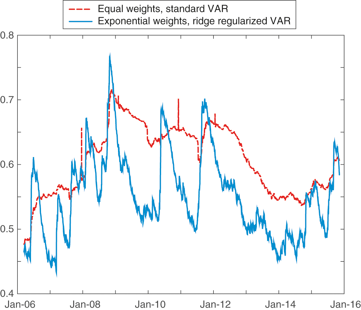
Using data from January 2005 to October 2015, we compute the total connectedness of the three banking systems – NA, the EU and ASEAN – over a rolling window of 300 days for the ten-year period from March 2006 to November 2015. Figures 1, 2 and 3 report the results for each of the three systems, comparing the original approach of Diebold and Yilmaz (2009) (dashed red lines) with the improved approach proposed in this paper (solid blue lines). Let us first observe that the two approaches demonstrate similar values and comparable behavior with regard to total connectedness. We can see that the use of ridge regularized VAR eliminates some of the outlying spurious peaks observed with the original method. The effect is present in all samples across the three regions and periods, but it is particularly evident in Figure 2 for the peaks after January 2011 and January 2012. When dimensionality is high, as in the case of the EU banking system, ordinary least squares estimates tend to have high variance as a result of overfitting. Ridge regression provides parameter estimates that have low variance across rolling windows, which is a manifestation of the model’s ability to better generalize across different samples. This is why we observe no sudden jumps in the total connectedness when we estimate our VAR coefficients using ridge regression. More evident is the effect of exponential smoothing, which makes peaks sharper and eliminates the plateau effect due to the persistence of the influence of a peak during the whole length of the rolling window. This is especially evident in Figure 1, where for the standard VAR method the peak in total connectedness observed just after January 2009 persists, creating a plateau that drops abruptly after 300 days in January 2010. Conversely, the exponential weighted ridge regularized method reveals a clear peak, reaching its maximum around January 2009, followed by a sharp decrease. We observe that the plateau effects in the standard VAR-equal-weights method sometimes completely hide peaks that are instead detected with the exponentially weighted ridge regularized method. This is the case for the late-2010 NA spillover peak, which is visible in Figure 3 only for the exponentially weighted ridge regularized method.
Note that in Diebold and Yilmaz (2009), where total connectedness in both equity index returns and equity index return volatilities was measured, the authors found that the return spillovers demonstrated “a gently increasing trend but no bursts, whereas volatility spillovers display[ed] no trend but clear bursts”. Our results in Figures 1, 2 and 3 indicate that applying exponential weights to the returns allows us to observe both trends and bursts in the return uncertainty spillovers.




A comparison between ASEAN, EU and NA total connectedness from the ridge regularized VAR models is presented in Figure 4, where major events are labeled on the graph when they occurred. The general shapes of the total connectedness of the three banking systems appear to be similar. Over the approximately ten-year period from March 2006 to November 2015, the values of NA’s total connectedness are generally higher than those of the EU and ASEAN banking systems, except in the following periods: 2006 to mid-2007, early 2011, early 2013 and mid-2014.
The fact that NA, EU and ASEAN banking systems have different levels of interconnectivity reflects the dissimilarities in the natures of the three banking systems. Our data set includes large banks operating at the national level (GICS code 40101010) that survived in the period from January 2005 to October 2015. Based on the GICS code and survival criteria, our NA system covers two countries (ten banks), the EU covers seventeen countries (sixty-six banks) and ASEAN covers five countries (thirty-nine banks). The two countries in the NA system (the United States and Canada) have banking regulations that are more similar than those of the seventeen countries in the EU or those of the five countries in ASEAN. In addition, the equities of the ten banks in NA trade on the same stock exchange – the NYSE – while those of the EU and ASEAN banks trade on different national stock exchanges. Finally, as banks tend to form business relationships with other banks that are in close proximity, both geographically and from a regulatory perspective, the number of interbank business activities in NA is likely to be higher than in the EU and ASEAN. These three factors contribute to stronger links and a higher possibility of spillovers among NA banks than among EU or ASEAN banks. For the above reasons, total connectedness in the NA system is generally higher than in the EU and ASEAN systems.
The number of banks in a system does not seem to be a factor that influences the level of total connectedness, as there is no relationship between the number of banks and total connectedness in a system. Note that the total connectedness metric is computed on a per-bank basis; it is the average of all pairwise connectedness in a system.
From visual inspection of Figure 4, we note that variations in total connectedness of the NA banking system seem to lead those of the EU and ASEAN systems, while the total connectedness of the EU system seems to lead that of the ASEAN system. This prompts us to perform causality tests on the total connectedness time series of the three banking systems in order to investigate how systemic uncertainty in each region influences the others as well as the lead–lag relationships among them.


| Net | |||
|---|---|---|---|
| information | |||
| Method | flow | ||
| Linear | 0.004722 | 0.001354 | 0.003369 |
| Nonlinear threshold | 0.005251 | 0.006711 | 0.001460 |
| Nonlinear threshold | 0.003980 | 0.002012 | 0.001968 |
| Nonlinear threshold | 0.004939 | 0.000561 | 0.004378 |
| Net | |||
| information | |||
| Method | flow | ||
| Linear | 0.017336 | 0.008931 | 0.008405 |
| Nonlinear threshold | 0.008789 | 0.005837 | 0.002953 |
| Nonlinear threshold | 0.005348 | 0.002305 | 0.003042 |
| Nonlinear threshold | 0.003150 | 0.002803 | 0.000348 |
| Net | |||
| information | |||
| Method | flow | ||
| Linear | 0.005659 | 0.003633 | 0.002026 |
| Nonlinear threshold | 0.005553 | 0.001262 | 0.004291 |
| Nonlinear threshold | 0.005960 | 0.000228 | 0.005732 |
| Nonlinear threshold | 0.004238 | 0.002118 | 0.002120 |
| Net | |||
|---|---|---|---|
| information | |||
| Method | flow | ||
| Linear | 0.008003 | 0.001255 | 0.006747 |
| Nonlinear threshold | 0.009204 | 0.009474 | 0.000271 |
| Nonlinear threshold | 0.017228 | 0.003196 | 0.014032 |
| Nonlinear threshold | 0.024087 | 0.002335 | 0.021752 |
| Net | |||
| information | |||
| Method | flow | ||
| Linear | 0.017200 | 0.003703 | 0.013497 |
| Nonlinear threshold | 0.010598 | 0.004354 | 0.006244 |
| Nonlinear threshold | 0.006509 | 0.006475 | 0.000034 |
| Nonlinear threshold | 0.002107 | 0.006805 | 0.004698 |
| Net | |||
| information | |||
| Method | flow | ||
| Linear | 0.022020 | 0.000619 | 0.021401 |
| Nonlinear threshold | 0.021641 | 0.002374 | 0.019267 |
| Nonlinear threshold | 0.022964 | 0.002900 | 0.020063 |
| Nonlinear threshold | 0.007488 | 0.000405 | 0.007083 |
5.2 Causality tests on regional total connectedness
In order to quantify the lead–lag relationships among the NA’s, EU’s and ASEAN’s total connectedness, we compute transfer entropy and information flow between the daily changes of total connectedness in the three regions for a one-day lag. Results are reported in Table 4. Transfer entropies are estimated using both the linear and the nonlinear approaches discussed in Section 4.2. We recall that the linear measure is equivalent to Granger causality, where a significant transfer entropy corresponds to a validated Granger causality relation. The nonlinear measures are computed for fluctuation bands at standard deviations (see Section 4.2). Observe that there is a significant information transfer between NA and EU, NA and ASEAN, and EU and ASEAN that, for the linear case, implies NA Granger causes EU, NA Granger causes ASEAN, and EU Granger causes ASEAN. We observe that the nonlinear estimation gives consistent results with the linear estimate for all values of , demonstrating the robustness of the result. We also observe that there are significant causal relations in the opposite direction. Given the extended time-lags between the three regions, it is fair to question whether a one-day time lag and a one-day time horizon will affect markets asymmetrically depending on their relative opening hours. We therefore test the flow of information across regions for a time horizon and lag of five days instead of one day. The results for the transfer entropies and information flow, performed for the entire period on nonoverlapping five-day returns, are reported in Table 5. We observe that the results are consistent with those for a one-day time horizon and lag reported in Table 4, the main difference being the lower statistical significance. This is expected because the time series for the five-day changes are five times shorter than those for daily changes.
6 Conclusion
We investigate regional and inter-regional uncertainty spillovers in the NA, EU and ASEAN banking systems during a period characterized by great regional and global financial stress (2005–15). Uncertainty and financial instability is quantified by means of total network connectedness, which we measure by improving on the method of Diebold and Yilmaz (2009). We demonstrate that exponential smoothing and ridge regression provide better-defined peaks in the temporal analysis and avoid the occurrence of some spurious peaks. We observe that the NA system appears to be consistently more interconnected than that of the EU, which in turn is more interconnected than the ASEAN network. Similarly to the previous analysis of Diebold and Yilmaz of other systems, our empirical analysis of the NA, EU and ASEAN banking networks shows that increased connectivity corresponds to periods of higher distress in the system. We observe that all large peaks of total network connectedness are associated with identifiable major exogenous events. Despite some of these events being related to specific regions, the effects are seen across all three banking systems, which reveal similar patterns of peaks and troughs in the variations of their total network connectedness. However, such variations are not perfectly synchronous across the regions, and causality patterns are discovered using transfer entropy. Our analysis reveals that the NA banking system is the most influential, having the largest effect on the other systems. However, feedback effects are measured with significant causal relations in the opposite direction as well. The results are demonstrated to be robust with respect to changes in the method used to compute the transfer entropy, changes in the values of parameters, and with respect to the use of daily or weekly returns in the analysis.
To summarize, the contribution of this paper is threefold. First, we improve the technical aspect of VAR estimation, allowing for better identification of events concentrated at specific times, which leads to a more accurate and insightful interpretation of the results. Second, we focus on connectedness in the banking sector, while previous studies based on the Diebold and Yilmaz (2009) methodology have analyzed networks of financial institutions. In particular, we analyze the NA, EU and ASEAN banking systems individually and show that, despite the regions’ being geographically distant, they are affected to varying degrees by major financial crisis events originating in dominant regions such as the NA and EU banking systems. Third, we perform a causality analysis on the regional connectedness time series generated using Diebold and Yilmaz’s method. Our analysis suggests that a regional disaggregated investigation has the advantage of introducing a predictive component to this methodology. While the network total connectedness measure identifies increases in regional uncertainty associated with major events that shake the markets, the causality relation between total connectedness in different regions – introduced in this paper – provides a quantitative characterization of the flow of uncertainty from region to region, which could be interpreted as the result of contagion. To the best of our knowledge, this causality analysis is the first of its kind.
In future, we will compare this approach with other information theoretic measures with the aim of finding a framework that is capable of qualifying financial uncertainty and its causal effects at all levels of aggregation, from a local single-variable perspective to a global world-market view.
Declaration of interest
The authors report no conflicts of interest. The authors alone are responsible for the content and writing of the paper.
Acknowledgements
T.A. and F.C. acknowledge the support of the UK Economic and Social Research Council (ESRC) in funding the Systemic Risk Centre (ES/K002309/1).
References
- Admati, A., DeMarzo, P., Hellwig, M., and Pfleiderer, P. (2013). Fallacies, irrelevant facts, and myths in the discussion of capital regulation: why bank equity is not socially expensive. Working Paper, Social Science Research Network (https://doi.org/10.2139/ssrn.2349739).
- Adrian, T., and Brunnermeier, M. K. (2016). CoVaR. American Economic Review 106, 1705–1741 (https://doi.org/10.1257/aer.20120555).
- Allen, F., and Gale, D. (2000). Financial contagion. Journal of Political Economy 108, 1–33 (https://doi.org/10.1086/262109).
- Alter, A., and Beyer, A. (2014). The dynamics of spillover effects during the European sovereign debt turmoil. Journal of Banking and Finance 42, 134–153 (https://doi.org/10.1016/j.jbankfin.2014.01.030).
- Bardoscia, M., Battiston, S., Caccioli, F., and Caldarelli, G. (2015). Debtrank: a microscopic foundation for shock propagation. PLoS ONE 10, 1–13 (https://doi.org/10.1371/journal.pone.0130406).
- Bardoscia, M., Battiston, S., Caccioli, F., and Caldarelli, G. (2017). Pathways towards instability in financial networks. Nature Communications 8, 14416 (https://doi.org/10.1038/ncomms14416).
- Barnett, L., Barrett, A., and Seth, A. (2009). Granger causality and transfer entropy are equivalent for Gaussian variables. Physical Review Letters 103, 238701 (https://doi.org/10.1103/PhysRevLett.103.238701).
- Battiston, S., Puliga, M., Kaushik, R., Tasca, P., and Caldarelli, G. (2012). Debtrank: too central to fail? Financial networks, the Fed and systemic risk. Scientific Reports 2, 1–6 (https://doi.org/10.1038/srep00541).
- Beale, N., Rand, D. G., Battey, H., Croxson, K., May, R. M., and Nowak, M. A. (2011). Individual versus systemic risk and the regulator’s dilemma. Proceedings of the National Academy of Sciences 108, 12 647–12 652 (https://doi.org/10.1073/pnas.1105882108).
- Billio, M., Getmansky, M., Lo, A., and Pelizzon, L. (2012). Econometric measures of connectedness and systemic risk in the finance and insurance sectors. Journal of Financial Economics 104, 535–559 (https://doi.org/10.1016/j.jfineco.2011.12.010).
- Birch, A., and Aste, T. (2014). Systemic losses due to counterparty risk in a stylized banking system. Journal of Statistical Physics 156, 998–1024 (https://doi.org/10.1007/s10955-014-1040-9).
- Brownlees, C., and Engle, R. (2016). Srisk: a conditional capital shortfall measure of systemic risk. Review of Financial Studies 30, 48–79 (https://doi.org/10.1093/rfs/hhw060).
- Bubák, V., Kočenda, E., and Žikeš, F. (2011). Volatility transmission in emerging European foreign exchange markets. Journal of Banking & Finance 35, 2829–2841 (https://doi.org/10.1016/j.jbankfin.2011.03.012).
- Caccioli, F., Shrestha, M., Moore, C., and Farmer, J. (2014). Stability analysis of financial contagion due to overlapping portfolios. Journal of Banking & Finance 46, 233–245 (https://doi.org/10.1016/j.jbankfin.2014.05.021).
- Caccioli, F., Farmer, J. D., Foti, N., and Rockmore, D. (2015). Overlapping portfolios, contagion, and financial stability. Journal of Economic Dynamics and Control 51, 50–63 (https://doi.org/10.1016/j.jedc.2014.09.041).
- Caccioli, F., Barucca, P., and Kobayashi, T. (2018). Network models of financial systemic risk: a review. Journal of Computational Social Science 1, 81–114 (https://doi.org/10.1007/s42001-017-0008-3).
- Caceres, C., Guzzo, V., and Segoviano, M. (2010). Sovereign spreads: global risk aversion, contagion or fundamentals? Working Paper, International Monetary Fund.
- Chau, F., and Deesomsak, R. (2014). Does linkage fuel the fire? The transmission of financial stress across the markets. International Review of Financial Analysis 36, 57–70 (https://doi.org/10.1016/j.irfa.2014.02.005).
- Claeys, P., and Vasicek, B. (2014). Measuring bilateral spillover and testing contagion on sovereign bond markets in Europe. Journal of Banking & Finance 46, 151–165 (https://doi.org/10.1016/j.jbankfin.2014.05.011).
- Cochrane, J. H. (2005). Time series for macroeconomics and finance. Unpublished manuscript, Graduate School of Business, University of Chicago.
- Cont, R., Moussa, A., and Santos, E. (2010). Network structure and systemic risk in banking systems. Working Paper, Social Science Research Network (https://doi.org/10.2139/ssrn.1733528).
- Corsi, F., Marmi, S., and Lillo, F. (2016). When micro prudence increases macro risk: the destabilizing effects of financial innovation, leverage, and diversification. Operations Research 64, 1073–1088 (https://doi.org/10.1287/opre.2015.1464).
- Degryse, H., and Nguyen, G. (2007). Interbank exposures: an empirical examination of systemic risk in the Belgian banking system. International Journal of Central Banking 3, 951–979.
- Demirer, M., Diebold, F. X., Liu, L., and Yilmaz, K. (2018). Estimating global bank network connectedness. Journal of Applied Econometrics 33(1), 1–15 (https://doi.org/10.1002/jae.2585).
- Diebold, F. X., and Yilmaz, K. (2009). Measuring financial asset return and volatility spillovers, with application to global equity markets. Economic Journal 119, 158–171 (https://doi.org/10.1111/j.1468-0297.2008.02208.x).
- Diebold, F. X., and Yilmaz, K. (2012). Better to give than to receive: predictive directional measurement of volatility spillovers. International Journal of Forecasting 28, 57–66 (https://doi.org/10.1016/j.ijforecast.2011.02.006).
- Diebold, F. X., and Yilmaz, K. (2014). On the network topology of variance decompositions: measuring the connectedness of financial firms. Journal of Econometrics 182, 119–134 (https://doi.org/10.1016/j.jeconom.2014.04.012).
- Dungey, D., Fry, R., Gonzales-Hermosillo, B., and Martin, V. (2005). Empirical modelling of contagion: a review of methodologies. Quantitative Finance 5, 9–24 (https://doi.org/10.1080/14697680500142045).
- Eisenberg, L., and Noe, T. (2001). Systemic risk in financial systems. Management Science 47, 236–249 (https://doi.org/10.1287/mnsc.47.2.236.9835).
- Fengler, M., and Gisler, K. (2015). A variance spillover analysis without covariances: what do we miss? Journal of International Money and Finance 51, 174–195 (https://doi.org/10.1016/j.jimonfin.2014.11.006).
- Fricke, D., and Lux, T. (2015). Core–periphery structure in the overnight money market: evidence from the e-mid trading platform. Computational Economics 45, 359–395 (https://doi.org/10.1007/s10614-014-9427-x).
- Fujiwara, I., and Takahashi, K. (2012). Asian financial linkage: macro-finance dissonance. Pacific Economic Review 17(1), 136–159 (https://doi.org/10.1111/j.1468-0106.2011.00575.x).
- Furfine, C. H. (2003). Interbank exposures: quantifying the risk of contagion. Journal of Money, Credit and Banking 35, 111–128 (https://doi.org/10.1353/mcb.2003.0004).
- Gai, P., and Kapadia, S. (2010). Contagion in financial networks. Proceedings of the Royal Society of London A 466(2120), 2401–2423 (https://doi.org/10.1098/rspa.2009.0410).
- Glasserman, P., and Young, H. P. (2016). Contagion in financial networks. Journal of Economic Literature 54, 779–831 (https://doi.org/10.1257/jel.20151228).
- Granger, C. W. (1988). Some recent development in a concept of causality. Journal of Econometrics 39, 199–211 (https://doi.org/10.1016/0304-4076(88)90045-0).
- Gruber, M. (1998). Improving Efficiency by Shrinkage: The James–Stein and Ridge Regression Estimators, Volume 156. CRC Press, Boca Rato, FL.
- Harris, R. J. (1985). A Primer of Multivariate Statistics, 2nd edn. Academic Press, Orlando, FL.
- Hoerl, A. E., and Kennard, R. W. (1970). Ridge regression: biased estimation for nonorthogonal problems. Technometrics 12, 55–67 (https://doi.org/10.1080/00401706.1970.10488634).
- Huang, X., Vodenska, I., Havlin, S., and Stanley, H. E. (2013). Cascading failures in bi-partite graphs: model for systemic risk propagation. Scientific Reports 3, 1–8.
- Iori, G., Jafarey, S., and Padilla, F. G. (2006). Systemic risk on the interbank market. Journal of Economic Behavior & Organization 61, 525–542 (https://doi.org/10.1016/j.jebo.2004.07.018).
- Klößner, S., and Wagner, S. (2014). Exploring all VaR orderings for calculating spillovers? Yes, we can: a note on Diebold and Yilmaz (2009). Journal of Applied Econometrics 29, 172–179 (https://doi.org/10.1002/jae.2366).
- Kobayashi, T., and Hasui, K. (2014). Efficient immunization strategies to prevent financial contagion. Scientific Reports 4, 3834 (https://doi.org/10.1038/srep03834).
- Lenzu, S., and Tedeschi, G. (2012). Systemic risk on different interbank network topologies. Physica A 391, 4331–4341 (https://doi.org/10.1016/j.physa.2012.03.035).
- Lucas, A., Schwaab, B., and Zhang, X. (2014). Conditional euro area sovereign default risk. Journal of Business & Economic Statistics 32, 271–28 (https://doi.org/10.1080/07350015.2013.873540).
- Lutkepohl, H. (2006). New Introduction to Multiple Time Series Analysis. Springer.
- McMillan, D., and Speight, A. (2010). Return and volatility spillovers in three euro exchange rates. Journal of Economics and Business 62, 79–93 (https://doi.org/10.1016/j.jeconbus.2009.08.003).
- Moghadam, R., and Vinals, J. (2010). Understanding financial interconnectedness. Policy Paper, International Monetary Fund.
- Müller, J. (2006). Interbank credit lines as a channel of contagion. Journal of Financial Services Research 29, 37–60 (https://doi.org/10.1007/s10693-005-5107-2).
- Musmeci, N., Aste, T., and Di Matteo, T. (2015). Risk diversification: a study of persistence with a filtered correlation-network approach. The Journal of Network Theory in Finance 1, 1–22 (https://doi.org/10.21314/JNTF.2015.005).
- Nier, E., Yang, J., Yorulmazer, T., and Alentorn, A. (2007). Network models and financial stability. Journal of Economic Dynamics and Control 31, 2033–2060 (https://doi.org/10.1016/j.jedc.2007.01.014).
- Pozzi, F., Di Matteo, T., and Aste, T. (2012). Exponential smoothing weighted correlations. European Physical Journal B 85(175), 1–21 (https://doi.org/10.1140/epjb/e2012-20697-x).
- Shiller, R. J. (2003). From efficient markets theory to behavioral finance. Journal of Economic Perspectives 17, 83–104 (https://doi.org/10.1257/089533003321164967).
- Sims, C. A. (1980). Macroeconomics and reality. Econometrica 48, 1–48 (https://doi.org/10.2307/1912017).
- Stock, J. H., and Watson, M. W. (2001). Vector autoregressions. Journal of Economic Perspectives 15, 101–115 (https://doi.org/10.1257/jep.15.4.101).
- Tedeschi, G., Mazloumian, A., Gallegati, M., and Helbing, D. (2001). Vector autoregressions. PloS ONE 12, e52749.
- Tikhonov, A. (1963). Solution of incorrectly formulated problems and the regularization method. Soviet Mathematics Doklady 5, 1035–1038.
- Tsay, R. S. (2010). Analysis of Financial Time Series. Wiley (https://doi.org/10.1002/9780470644560).
- Upper, C. (2011). Simulation methods to assess the danger of contagion in interbank markets. Journal of Financial Stability 7, 111–125 (https://doi.org/10.1016/j.jfs.2010.12.001).
- Upper, C., and Worms, A. (2004). Estimating bilateral exposures in the German interbank market: is there a danger of contagion? European Economic Review 48, 827–849 (https://doi.org/10.1016/j.euroecorev.2003.12.009).
Only users who have a paid subscription or are part of a corporate subscription are able to print or copy content.
To access these options, along with all other subscription benefits, please contact info@risk.net or view our subscription options here: http://subscriptions.risk.net/subscribe
You are currently unable to print this content. Please contact info@risk.net to find out more.
You are currently unable to copy this content. Please contact info@risk.net to find out more.
Copyright Infopro Digital Limited. All rights reserved.
As outlined in our terms and conditions, https://www.infopro-digital.com/terms-and-conditions/subscriptions/ (point 2.4), printing is limited to a single copy.
If you would like to purchase additional rights please email info@risk.net
Copyright Infopro Digital Limited. All rights reserved.
You may share this content using our article tools. As outlined in our terms and conditions, https://www.infopro-digital.com/terms-and-conditions/subscriptions/ (clause 2.4), an Authorised User may only make one copy of the materials for their own personal use. You must also comply with the restrictions in clause 2.5.
If you would like to purchase additional rights please email info@risk.net
