Journal of Risk
ISSN:
1465-1211 (print)
1755-2842 (online)
Editor-in-chief: Farid AitSahlia

A new dynamic hedging model with futures: the Kalman filter error-correction model
Need to know
- This paper proposes a hedging model that combines the Kalman filter with error correction, namely the Kalman filter error-correction model (KF-ECM).
- This paper uses daily data of the Taiwan Capitalization Weighted Stock Index (TAIEX) and its futures from July 21, 1998 to March 27, 2019 to evaluate the hedging performance of KF-ECM. In addition, we compare the hedge effectiveness between KF-ECM and other hedging models by in-sample and out-of-sample prediction.
- The KF-ECM is regarded as a robust method to estimate the optimal hedge ratio without linearity and normality assumptions
Abstract
This paper proposes a new econometric model for the estimation of optimal hedge ratios (HRs): the Kalman filter error-correction model (KF–ECM). This paper proposes a new econometric model for the estimation of optimal hedge ratios (HRs): the Kalman filter error-correction model (KF–ECM). When we construct a hedging model involving a stock index and its futures, the KF state-space model is used to extract the single best latent common trend between the stock index and its futures. After the best common trend has been obtained, we substitute it into an ECM to estimate the HR; therefore, the KF–ECM combines the merits of error correction and state-space hedge models. This paper uses daily data from the Taiwan Capitalization Weighted Stock Index and its futures from July 21, 1998 to March 27, 2019 to evaluate the hedging performance of the KF–ECM. The study uses a hedging effectiveness (HE) index to compare the performance of the KF–ECM with that of other hedging models, including ordinary least squares, generalized autoregressive conditional heteroscedasticity and cointegrating ECMs. The empirical results of testing both in-sample and out-of-sample data show the KF–ECM to be more effective than other hedging models. The results also demonstrate that, regardless of the financial crisis, the HE of the KF–ECM remains the highest among all the models.
Introduction
1 Introduction
Since stock index futures were introduced to the market in the late 1970s, they have become popular hedging instruments. Due to growing fluctuations in stock markets, it is increasingly important to choose the optimal hedging strategy. Early studies used traditional ordinary least squares (OLS) regressions to estimate optimal hedge ratios (HRs) and hedging effectiveness (HE) (Johnson 1960; Ederington 1979). Although the OLS method identifies the relationship between a stock index and its futures, it has two major drawbacks. First, the stock index and its futures series exhibit nonstationary and conditional volatilities that are often neglected by the OLS model. When the nonstationary, conditional volatilities of a stock index portfolio and its futures are not taken into consideration, the HR estimated by the OLS method can lead to a suboptimal hedging decision. Second, the OLS approach involves a one-time hedging decision and does not allow for any adjustment in the HR once this decision has been made. When new information becomes available, investors using the OLS hedging model cannot immediately adjust their hedging decisions.
To represent the dynamic nature of HRs, most recent studies have employed autoregressive conditional heteroscedasticity (ARCH), generalized autoregressive conditional heteroscedasticity (GARCH), cointegration or state-space models (SSMs).11 1 Chen et al (2003) and Lien and Tse (2002) provide excellent reviews of HR research. ARCH-based models consider time-varying volatility and are widely used in estimating optimal HRs.22 2 Holmes (1996), Baillie and Myers (1991), Kroner and Sulten (1993) and Hsu et al (2008) use different ARCH and GARCH models to estimate time-varying HRs under conditional heteroscedasticity. Although the conditional heteroscedasticity hedging estimation method allows the HR to change over time, Miffre (2004) found that ARCH and GARCH models provide limited improvement to HE. In contrast, Ghosh (1993a,b) proposed an error-correction hedging model that considers the nonstationary nature of financial time series. Ghosh (1993a,b) uses the Engle–Granger two-step method to estimate the cointegrating relationship between stock portfolios and futures. When a cointegrating relationship exists, the optimal HR can be estimated through an error-correction regression. The advantage of the cointegration method is that, when the stock price index and futures possess unit roots, it can avoid spurious regression (Ferson et al 2003). However, even if the HRs in the error-correction regression are easy to compute, this model cannot outperform other hedging models. The disadvantage of the error-correction hedging model is that information cannot be updated during the estimation process. This leads to an inaccurate calculation of the long-term relationship between a stock index and its futures: a serious drawback considering that accurate identification of the long-run relationship is critical to HE.
The third approach to estimating the HR is an SSM. Hatemi-J and Roca (2006) introduced the Kalman filter (KF) model for estimating a time-varying HR. Lee et al (2006) estimated HRs with a random-coefficient autoregressive regime-switching model. Although SSMs demonstrate better efficiency, the drawbacks of traditional state-space hedging models are twofold. First, traditional time-varying SSMs (see, for example, Hatemi-J and Roca 2006; Lee et al 2006) use the stock index as the regressand and its futures as the regressor; thus, they extract the trend between the stock index and its futures. When the stock index and futures follow different trends, traditional SSMs cannot obtain the single best common trend. Second, although SSMs exhibit better efficiency in the autoregressive moving average (ARMA) process, the assumption of stationarity of the regressand and regressors is crucial to the estimation of HRs (Harvey 1990; Kim and Nelson 1999). The violation of this stationarity by the regressand and regressors can cause inconsistency in the estimation of the HR, resulting in the utilization of a suboptimal HR.33 3 Please refer to Chang et al (2009) for further discussion of the KF.
Many empirical studies have compared methods of estimating HRs. Benet (1992) used the OLS method to estimate the HR for the exchange rate futures of eight countries and observed a significant decrease in hedging performance from in-sample to out-of-sample estimation. Park and Switzer (1995) compared the HE of a conventional OLS model, an OLS model with cointegration and a bivariate GARCH model. They did so by examining Standard & Poor’s 500 (S&P 500) and Toronto 35 index futures. Of the three models, the bivariate GARCH model had the best HE. Holmes (1996) assessed estimation methods for the optimal HR of the Financial Times Stock Exchange 100 (FTSE 100) stock futures using OLS, cointegration and GARCH models. The optimal HR estimated by OLS outperformed those estimated via the more advanced econometric techniques of cointegration and GARCH. Ghosh (1993b) studied S&P 500 futures with the cointegration model and concluded that the traditional OLS approach could not be applied to the stock index and futures data because they could be nonstationary. When unit roots exist in the stock index and its futures, an OLS method may underestimate the HR. Hatemi-J and Roca (2006) examined the HE of Australian equity and futures using the time-varying parameter Kalman filter (TVPKF). The TVPKF outperformed the conventional OLS model. According to these empirical results, a single dominant model does not exist for optimizing dynamic hedging strategies.
This paper proposes a new method of determining the optimal HR: the Kalman filter error-correction model (KF–ECM). When we construct a hedging model involving a stock index and its futures, the Kalman filter state-space model (KF–SSM) (that is, the new econometric methodology proposed by Chang et al (2009)) is used to extract the single best latent common trend between the stock index and its futures. The difference between the long-run relationships estimated by the traditional maximum likelihood error-correction method (ML–ECM) and the KF–SSM is that the KF–SSM procedure allows for information on the stock index and its futures to be updated. After the best common trend has been obtained, we substitute it into an ECM to estimate the HR. Since the KF–ECM combines the merits of error-correction and state-space hedge models, we expect it to exhibit better HE than other, more traditional methods (see, for example, Baillie and Myers 1991; Ederington 1979; Ghosh 1993a,b; Holmes 1996).
In practice, the HR depends on the conditional information about the spot returns and their futures returns; therefore, when the conditional information changes over time, the HR also changes. Hedging strategies that employ an invariant HR are inadequate for multiperiod hedging (Benet 1992; Lien and Luo 1993). To compare the HE under time-varying circumstances, this study employs a rolling regression (moving window) to calculate the HE index (HEI), as proposed by Park and Switzer (1995). Rolling regression is a common forecasting method in time series analysis. Each time we perform a rolling regression, we add a period of data from the prediction sample. After the estimation is complete, we compare the predicted value with the actual value. We repeat this step until all data from the prediction samples has been added to the estimate. We then use the rolling regression to compare the out-of-sample performance of all examined hedging models.44 4 The hedging models include the OLS, GARCH, traditional TVPKF and ECMs.
This study contributes to the literature in two ways. First, we provide evidence that in high-dimensional applications, where some series are more important than others in driving the trend, the KF–ECM method provides a superior way of extracting common trends. When we use the KF–ECM to extract latent common trends, the KF method can set different weights according to the importance of the latent trends and extract the single best trend. By contrast, the ML–ECM assigns the same weight to all possible latent common trends and extracts the best trends; no restriction is placed on the number of trends. In high-dimensional financial applications and when a single best trend is required, the KF–ECM may be a more effective approach than the ECM. Second, the KF–ECM uses maximum likelihood estimation (MLE) to obtain the parameters. Even if the distributions of the data have thick tails, reasonable parameter estimates can be obtained. By contrast, ARCH and GARCH hedge models may be challenged by order selection with conditional correlations. HRs can be biased when the ARCH and GARCH models are incorrectly specified. For these reasons, investors may adopt the KF–ECM as a more accurate method for the estimation of the optimal HR.
The remainder of this paper is organized as follows. Section 2 describes the characteristics and estimation methods of the KF–ECM hedging model. Section 3 presents the empirical results for the KF–ECM, compares the common trends extracted using MLE and KF–SSM, and examines the effectiveness of the different hedging models. Finally, Section 4 presents the conclusions of this study.
2 The Kalman filter error-correction hedging model
Kalman (1960) proposed an SSM known as the KF for computing the optimal parameters of an unobserved trend at time based on the available information at . The KF has been used to analyze dynamic time series in such fields as aeronautical and electrical engineering.55 5 Refer to Harvey (1990), Hamilton (1994) and Kim and Nelson (1999) for their excellent surveys. Although the KF allows the state variable estimate to be continually updated as new observations become available, the latent trend must be a stationary series. To mitigate this drawback, Chang et al (2009) considered an SSM with integrated time series,
| (2.1) | ||||
| (2.2) |
where is a scalar latent variable with fixed initial value ; is an observable time series; and and are sequences of independent and identically distributed (iid) errors with means of zero and variances of and , respectively.66 6 The variance of is set to be unity for the identification of parameter . The other conditions imposed in the KF model are standard. For convenience, we may assume that , where is the stock index and represents the stock index futures. and are coefficients and errors, respectively. Equations (2.1) and (2.2) are referred to as the measurement and the state-space equations, respectively. Let be the observed variable vector, which can be represented by an unobserved variable . The KF–SSM proposed by Chang et al (2009) was used to extract the best common stochastic trends between and .
The following two stages are proposed to estimate the Kalman state space with the KF–ECM.
- (1)
Extract the common trend using the KF–SSM.
Unlike traditional cointegration estimation procedures, the KF requires three steps: prediction, estimation and updating.77 7 Estimation using the Engle–Granger or Johansen procedures does not involve updating steps. In the prediction step, we use the linear conditional expectations of the mean and variance,
(2.3) (2.4) where is a sigma field generated by . The mean square error (MSE) of prediction using (2.3) and (2.4) is defined below:
(2.5) (2.6) When the prediction value is obtained, the cointegrated SSM is decomposed into permanent and transitory components (as in Chang et al 2009):
where and are permanent and transitory components, respectively. Because is a function of and is a series with an I(1) stochastic common trend, the common trend can be extracted using MLE:
(2.7) (2.8) where is the steady-state value of . When the prediction error is obtained through MLE, it contains new information about beyond what is found in information set . The estimation of is updated using the updating equation:
(2.9) and (2.10) The authors repeat these three steps for . Any given values of and correspond with steady-state values of and that are denoted by and . The unobserved state-space parameter can be extracted iteratively.
After the common trend has been estimated, the measurement equation (2.1) can be rewritten as
(2.11) (2.12) Because is a latent variable, we rewrite as a function of (2.12),
(2.13) Substituting (2.13) into (2.11), the stochastic common trend between the stock index and futures can be expressed as
(2.14) - (2)
Substitute the common trend in (2.14) into the ECM
(2.15) where and are daily changes in the futures price and spot price , and is the HR. The new two-stage method for estimating the HR is called the KF–ECM estimator.
3 Methods and empirical results
This paper examines the stock indexes of the nineteen industries included in the Taiwan Stock Exchange (TWSE). The sample comprises daily data from July 21, 1998 to March 27, 2019, a period that includes both the global financial crisis and the European debt crisis.88 8 Weekends and holidays have been deleted from the series. Table 1 shows the percentage distribution of the industries in the Taiwan Capitalization Weighted Stock Index (TAIEX).
| Percentage | Percentage | ||
|---|---|---|---|
| Industry | (%) | Industry | (%) |
| Electrical | 54.6 | Building material | 1.1 |
| and construction | |||
| Finance and | 12.5 | Trading and | 1.0 |
| insurance | consumer goods | ||
| Plastic | 8.3 | Rubber | 1.0 |
| Iron and steel | 3.3 | Electrical machinery | 0.8 |
| Shipping and | 2.4 | Automobile | 0.6 |
| transportation | |||
| Others | 1.8 | Electrical and cable | 0.4 |
| Textile | 1.5 | Glass and ceramic | 0.3 |
| Chemical and | 1.5 | Tourism | 0.3 |
| biotechnology | |||
| Food | 1.3 | Paper and pulp | 0.3 |
| Cement | 1.1 |
Table 6 presents the augmented Dickey–Fuller (ADF) unit test results. For the null hypothesis of a unit root, the level series cannot reject the null hypothesis. When we apply the ADF test for the first difference series, the ADF -statistic indicates the rejection of the null hypothesis of a unit root. Therefore, unit roots exist in all nineteen industrial series.
3.1 Extracting common trends in the TAIEX index
This paper uses the nineteen main industrial weighted stock price indexes that comprise the TAIEX to illustrate how the KF–SSM extracts common stochastic trends shared by all series. Parameter estimates and their standard errors for (garnered using the KF–SSM) are given in Table 2, indicating how unobserved common stochastic trends affect each industrial stock index.


| Standard | Standard | ||||
|---|---|---|---|---|---|
| Estimate | error | Estimate | error | ||
| 0.0548 | 0.0008 | 0.0622 | 0.0009 | ||
| 0.0790 | 0.0012 | 0.0615 | 0.0009 | ||
| 0.0627 | 0.0009 | 0.0700 | 0.0010 | ||
| 0.0714 | 0.0010 | 0.0654 | 0.0010 | ||
| 0.0563 | 0.0008 | 0.0527 | 0.0008 | ||
| 0.0469 | 0.0007 | 0.0578 | 0.0009 | ||
| 0.0542 | 0.0008 | 0.0820 | 0.0012 | ||
| 0.0475 | 0.0007 | 0.0594 | 0.0009 | ||
| 0.0622 | 0.0009 | 0.0604 | 0.0009 | ||
| 0.0546 | 0.0008 |
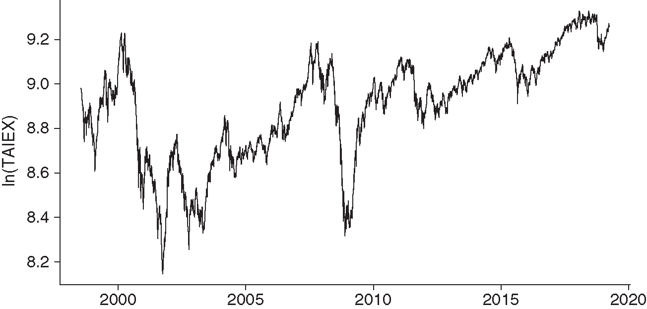
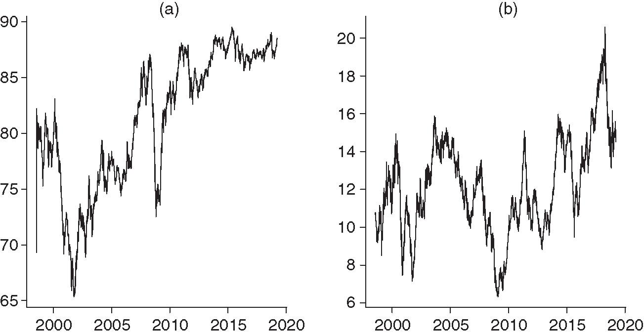
Figures 1 and 2 show the TAIEX and the common trends extracted from the nineteen industrial stock indexes using the KF–SSM and the traditional ML–ECM. Figure 2 reveals that the common trends extracted by the two methods are considerably different. Because the KF–SSM requires strong identification conditions in the optimization process, the common trend extracted by the KF–SSM cannot be numerically similar to the stock price index.99 9 Because we restrict and covariance to be diagonal for identification, we cannot reproduce the TAIEX exactly. However, the common trend extracted by the KF–SSM looks similar to the trend seen in the TAIEX. By contrast, the common trend extracted by the ML–ECM does not resemble the TAIEX.
The KF–SSM provides a technique for extracting a common stochastic trend with weights that are chosen by the principles of MLE, absolving the need for industries to be weighted by market capitalization or trading volume. When the trend of a market index is primarily driven by specific industries, the KF–SSM automatically increases the weight of these industries, providing an effective means of extracting a common trend. The ML–ECM, however, is designed to place the same weight on each industrial index, meaning that it may yield a poor result in our case. The TAIEX is a market-value-weighted index. The resemblance between the TAIEX and the common trend extracted by the KF–SSM suggests that the trend observed in the Taiwan stock market is indeed driven specifically by large-market-value industries.
3.2 Performance of the KF–ECM
This section evaluates the hedging performance of models of different specifications.. To simplify our analysis, we assume that the only hedging instruments in the stock market are futures contracts. The hedge portfolio consists of spots and futures, and transaction costs do not exist. When investors engage in hedging activity, they hold a short futures position in their investment. For comparison, the HR is defined as
| (3.1) |
The HR can be made dynamic by considering a multiperiod model where the HR may vary in different time periods, acknowledging that the optimal HR depends on time. After the HR is obtained, we calculate the HE as proposed by Park and Switzer (1995),
| (3.2) |
where and denote the variance of portfolios that are hedged using futures and unhedged, respectively. The HE approaches 1 if the hedging scheme is effective.
We use daily data of the TAIEX and its futures from July 21, 1998 to March 27, 2019.1010 10 Because Taiwan stock futures transactions began in July 1998, we choose data starting from July 21, 1998. We choose this sample period because notable financial crises such as the global financial crisis and the European debt crisis occurred during this time. We then compare the HE of the different models. The hedging models considered in this paper are the OLS, the GARCH(1,1), the time-varying parameter KF (TVPKF), the ML–ECM and the KF–ECM.
- (1)
OLS model (Ederington 1979),
(3.3) where is the HR and . A major problem with the OLS model is its dependence on unconditional information. As the dynamic HR depends on conditional information on the stock index and futures returns, the dynamic HR estimated from an OLS regression will not be optimal.
- (2)
The GARCH(1,1) model (Baillie and Myers 1991; Holmes 1996),
(3.4) where is the information set at time , is conditional variance and is unconditional variance. GARCH(1,1) can take into account the heteroscedastic nature of the errors in (3.4). The minimum HR is .
- (3)
The TVPKF model (Hatemi-J and Roca 2006),
(3.5) where . is the HR. The distinguishing factor of the TVPKF is its use of stock-index and stock-futures levels to calculate the HR.
- (4)
The ML–ECM (Ghosh 1993a,b),
(3.6) First, the cointegrating parameter in (3.6) is calculated using the Johansen MLE method. Second, the error correction (3.7) is estimated through OLS,
(3.7) where is the period residual of the cointegrating relationship estimated through MLE. The HR is equal to . Although both HRs are calculated using the variations in TAIEX and TAIEX futures, the main difference between (2.15) and (3.7) is that the KF–SSM procedure allows for information to be updated during the estimation process, whereas the ML–ECM does not. The two prediction errors
are not equal. (See Chang et al (2009) for detailed differences in error-correction representation between the KF–ECM and the ML–ECM.)
| Hedging | Error | ||||
|---|---|---|---|---|---|
| methods | OLS | GARCH(1,1) | TVPKF | correction | KF–ECM |
| Average variances | 1052.167 | 1094.937 | 2465.2296 | 848.139 | 832.496 |
| after hedging | |||||
| Variance reduction | 88.099% | 88.052% | 72.111% | 90.414% | 90.61% |
| improvement |
Regarding the choice of lagged periods for the ML–ECM and the KF–SSM, we choose one and four optimal lagged periods separately ( and ), as suggested by the Bayesian information criterion, for all and . The ADF unit root test is employed to test the TAIEX and the TAIEX futures series because we use the cointegrating model to estimate HE. ADF test results are presented in Table 7. We cannot reject the null hypothesis of the presence of a unit root in either the TAIEX or its futures series.
The parameter estimates generated by the various hedging models are presented in Table 8. Table 3 summarizes the results of the in-sample comparison of the HE of the different hedging models. The in-sample comparison suggests that the KF–ECM hedging model exhibits higher HE than conventional models. These results indicate that the KF–ECM hedging model is the most effective at minimizing the variance of hedged portfolios.
| Hedging | Error | ||||
|---|---|---|---|---|---|
| methods | OLS | GARCH(1,1) | TVPKF | correction | KF–ECM |
| SSR after hedging | 801.507 | 843.606 | 1929.848 | 663.123 | 652.083 |
| SSR reduction | 92.305% | 91.908% | 81.557% | 93.639% | 93.745% |
| improvement |
| Hedging | Error | ||||
|---|---|---|---|---|---|
| methods | OLS | GARCH(1,1) | TVPKF | correction | KF–ECM |
| SSR after hedging | 1003.808 | 1021.016 | 2074.969 | 801.34 | 800.759 |
| SSR reduction | 89.625% | 89.481% | 78.969% | 91.738% | 91.745% |
| improvement |
| Level | First-order difference | |||
| -statistic | -value | -statistic | -value | |
| Food | 1.160 | 0.939 | 72.529 | 0.000 |
| Plastic | 0.518 | 0.834 | 68.738 | 0.000 |
| Rubber | 0.003 | 0.684 | 67.134 | 0.000 |
| Tourism | 0.618 | 0.859 | 71.858 | 0.000 |
| Textile | 0.134 | 0.726 | 69.075 | 0.000 |
| Glass and ceramic | 1.161 | 0.226 | 68.980 | 0.000 |
| Chemical and biotechnology | 0.593 | 0.460 | 63.864 | 0.000 |
| Finance and insurance | 1.422 | 0.145 | 70.321 | 0.000 |
| Shipping and transportation | 0.776 | 0.383 | 65.623 | 0.000 |
| Cement | 0.091 | 0.661 | 51.250 | 0.000 |
| Trading and consumer goods | 0.466 | 0.518 | 70.984 | 0.000 |
| Iron and steel | 0.167 | 0.629 | 69.146 | 0.000 |
| Other | 0.810 | 0.895 | 67.536 | 0.000 |
| Building material and construction | 1.385 | 0.157 | 62.581 | 0.000 |
| Electrical machinery | 0.271 | 0.758 | 67.756 | 0.000 |
| Electrical and cable | 1.633 | 0.097 | 67.175 | 0.000 |
| Electrical | 0.047 | 0.672 | 67.673 | 0.000 |
| Automobile | 0.180 | 0.637 | 67.912 | 0.000 |
| Paper and pulp | 0.764 | 0.386 | 65.952 | 0.000 |
| Level | First-order difference | |||
| -statistic | -value | -statistic | -value | |
| TAIEX | 1.602 | 0.686 | 30.601 | 0.000 |
| TAIEX futures | 1.882 | 0.341 | 30.665 | 0.000 |
| OLS | GARCH | TVPKF | MLE–ECM | KF–ECM | |||
|---|---|---|---|---|---|---|---|
| 0.1008 | 0.8588 | 16.142 | 16.142 | 90.2619 | |||
| (0.4512) | (0.03456) | (3.1201) | (3.1201) | (0.73) | |||
| 0.8373 | 0.9994 | 0.9982 | 0.9994 | 90.1324 | |||
| (0.0043) | (0.0002) | (0.0004) | 0.0004 | (0.729) | |||
| 15.5990 | 0.0725 | 0.1198 | |||||
| (2.8670) | (0.4051) | (0.4016) | |||||
| 0.0735 | 0.1622 | 0.1264 | |||||
| (0.0073) | (0.0089) | (0.0096) | |||||
| 0.9122 | 0.8526 | 0.8538 | |||||
| (0.0087) | (0.0039) | (0.0039) | |||||
| 0.2053 | 0.2811 | ||||||
| (0.0132) | (0.0153) | ||||||
| 0.2334 | 0.305 | ||||||
| (0.012) | (0.014) | ||||||
| 0.1292 | |||||||
| (0.0154) | |||||||
| 0.1299 | |||||||
| (0.0143) | |||||||
| 0.0964 | |||||||
| (0.015) | |||||||
| 0.0894 | |||||||
| (0.0139) | |||||||
| 0.473 | |||||||
| (0.0134) | |||||||
| 0.0373 | |||||||
| (0.0124) |
Hedging models that achieve strong in-sample performances do not necessarily perform strongly out-of-sample. Therefore, it is necessary to determine whether the KF–ECM also exhibits a satisfactory out-of-sample hedging performance. To compare the model’s out-of-sample HE, we use a rolling regression and the out-of-sample prediction technology proposed by Chiu et al (2004) and Zivot and Wang (2006). First, we separate the sample period into two subsamples. The first subsample is from July 21, 1998 to December 31, 2006, and the second is from January 1, 2007 to January 19, 2015. We use the second subsample for out-of-sample forecasting. Because the second set of samples encompasses the period of the global financial crisis, we can compare the HE of all models during a period of serious financial crisis.1111 11 The global financial crisis occurred from 2007 to 2009. The European sovereign debt crisis began in 2008 with the collapse of Iceland’s banking system, and the crisis peaked between 2010 and 2012. The first subsample is used to estimate the HR. After the HR has been obtained, we calculate the HE. Next, we add one sample point from the second subsample into the first subsample and repeat all previous steps to calculate another HE value. We repeat all the previous steps until data from the second subsample has been added. After the HE has been calculated for the remaining subsample, we compute the HEIs,
| (3.8) |
where is the number of sample points in the second subsample. Finally, we compare the HEIs of all the hedging models. A HEI value close to 1 indicates that the hedging model has given a highly dynamic hedging performance.
Table 4 illustrates the measure of dynamic HE for the four examined hedging models. The results reveal that the KF–ECM outperformed the other hedging models in terms of its HE. Based on the in-sample and out-of-sample results, the KF–ECM may be useful for optimizing HE.
In addition to the first data segmentation, this study uses another grouping method. As before, we separate all data into two subsamples. The first subsample period is the same (July 21, 1998 to December 31, 2006), whereas the second subsample period is extended to span from January 19, 2015 to March 28, 2019. Table 5 shows the dynamic HE of the four examined hedging models. These results demonstrate that the HE of the KF–ECM remains the highest among all the models. Regardless of the financial crisis, the HR estimated by the KF–ECM exhibited higher HE than the level achieved by the other models.
4 Conclusion
This paper proposes a hedging model that combines the KF with error correction, namely the KF–ECM. We compare the HE of the KF–ECM with that of four other models: the dynamic OLS, the GARCH(1,1), the TVPKF and an error-correction hedging model. The KF–ECM exhibits greater HE than any other model, according to both in-sample and out-of-sample evidence. Compared with the other models, the improvement in HE offered by the KF–ECM is small; even so, it can still be regarded as a robust method of estimating the HR. In contrast with the ML–ECM, the KF–ECM method does not require linearity and normality assumptions. Even if the distributions of the data have thick tails, reasonable parameter estimates can be obtained using the KF–ECM. The KF–ECM can be a valuable tool for investors to use in dynamic hedging.
Although the KF–ECM boasts a highly dynamic HE, this method has two limitations. First, numerical optimization is required to calculate the parameters. Because much complexity and necessary computing time result from a large number of parameters, we must set restrictions on the parameters when estimating. Second, when estimating the HR, the KF–ECM does not consider possible transaction costs. Chen et al (2003) indicated that transaction costs do affect the optimal HR.
In future research, two research directions can be pursued. First, transaction costs can be factored into the KF–ECM to explore their effect on the optimal HR. Second, because the KF–ECM can extract the single best trend from multiple portfolios, researchers can explore the HE of the KF–ECM when expanding hedging instruments from single-index futures to multiple-asset portfolios.
Declaration of interest
The authors report no conflicts of interest. The authors alone are responsible for the content and writing of the paper.
References
- Baillie, R., and Myers, R. (1991). Bivariate GARCH estimation of the optimal commodity futures hedge. Journal of Applied Econometrics 6(2), 109–124 (https://doi.org/10.1002/jae.3950060202).
- Benet, B. A. (1992). Hedge period length and ex-ante futures hedging effectiveness: the case of foreign-exchange risk cross hedges. Journal of Futures Markets 12(2), 163–175 (https://doi.org/10.1002/fut.3990120205).
- Chang, Y., Miller, J., and Park, J. (2009). Extracting a common stochastic trend: theory with some applications. Journal of Econometrics 150(2), 231–247 (https://doi.org/10.1016/j.jeconom.2008.12.007).
- Chen, S., Lee, C., and Shrestha, K. (2003). Futures hedge ratios: a review. Quarterly Review of Economics and Finance 43(3), 433–465 (https://doi.org/10.1016/S1062-9769(02)00191-6).
- Chiu, C., Wei, C., Wu, P., and Chiou, J. (2004). The research of direct hedging strategies for TAIFEX and MSCI stock index futures. Commerce and Management Quarterly 5(2), 169–184.
- Ederington, L. (1979). The hedging performance of the new futures markets. Journal of Finance 34(1), 157–170 (https://doi.org/10.1111/j.1540-6261.1979.tb02077.x.).
- Ferson, W., Sarkissian, S., and Simin, T. (2003). Spurious regressions in financial economics? Journal of Finance 58(4), 1393–1413 (https://doi.org/10.1111/1540-6261.00571).
- Ghosh, A. (1993a). Cointegration and error correction models: intertemporal causality between index and futures prices. Journal of Futures Markets 13(2), 193–198 (https://doi.org/10.1002/fut.3990130206).
- Ghosh, A. (1993b). Hedging with stock index futures: estimation and forecasting with error correction model. Journal of Futures Markets 13(7), 733–752 (https://doi.org/10.1002/fut.3990130703).
- Hamilton, J. (1994). Time Series Analysis. Princeton University Press.
- Harvey, A. C. (1989). Forecasting, Structural Time Series Models and the Kalman Filter. Cambridge University Press.
- Hatemi-J, A., and Roca, E. (2006). Calculating the optimal hedge ratio: constant, time varying and the Kalman Filter approach. Applied Economics Letters 13(5), 293–299 (https://doi.org/10.1080/13504850500365848).
- Holmes, P. (1996). Stock index futures hedging: hedge ratio estimation, duration effects, expiration effects and hedge ratio stability. Journal of Business Finance and Accounting 23(1), 63–77 (https://doi.org/10.1111/j.1468-5957.1996.tb00402.x).
- Hsu, C., Tseng, C., and Wang, Y. (2008). Dynamic hedging with futures: a copula-based GARCH model. Journal of Futures Markets 28(11), 1095–1116 (https://doi.org/10.1002/fut.20345).
- Kim, C.-J., and Nelson, C. R. (1999). State-Space Models with Regime Switching: Classical and Gibbs-Sampling Approaches with Applications. MIT Press, Cambridge, MA.
- Kroner, K., and Sultan, J. (1993). Time-varying distributions and dynamic hedging with foreign currency futures. Journal of Finance and Quantitative Analysis 28(4), 535–551 (https://doi.org/10.2307/2331164).
- Lee, H., Yoder, J., Mittelhammer, R., and McCluskey, J. (2006). A random coefficient autoregressive Markov regime switching model for dynamic futures hedging. Journal of Futures Markets 26(2), 103–129 (https://doi.org/10.1002/fut.20193).
- Lien, D., and Luo, X. (1993). Estimating multiperiod hedge ratio in cointegrated markets. Journal of Futures Markets 13(8), 909–920 (https://doi.org/10.1002/fut.3990130808).
- Lien, D., and Tse, Y. (2002). Some recent developments in futures hedging. Journal of Economic Surveys 16(3), 357–396 (https://doi.org/10.1111/1467-6419.00172).
- Miffre, J. (2004). Conditional OLS minimum variance hedge ratios. Journal of Futures Markets 24(10), 945–964 (https://doi.org/10.1002/fut.20116).
- Park, T., and Switzer, L. (1995). Bivariate GARCH estimation of the optimal hedge ratios for stock index futures: a note. Journal of Futures Markets 15(1), 61–67 (https://doi.org/10.1002/fut.3990150106).
- Zivot, E., and Wang, J. (2006). Modeling Financial Time Series with S-PLUS. Springer (https://doi.org/10.1007/978-0-387-32348-0).
Only users who have a paid subscription or are part of a corporate subscription are able to print or copy content.
To access these options, along with all other subscription benefits, please contact info@risk.net or view our subscription options here: http://subscriptions.risk.net/subscribe
You are currently unable to print this content. Please contact info@risk.net to find out more.
You are currently unable to copy this content. Please contact info@risk.net to find out more.
Copyright Infopro Digital Limited. All rights reserved.
As outlined in our terms and conditions, https://www.infopro-digital.com/terms-and-conditions/subscriptions/ (point 2.4), printing is limited to a single copy.
If you would like to purchase additional rights please email info@risk.net
Copyright Infopro Digital Limited. All rights reserved.
You may share this content using our article tools. As outlined in our terms and conditions, https://www.infopro-digital.com/terms-and-conditions/subscriptions/ (clause 2.4), an Authorised User may only make one copy of the materials for their own personal use. You must also comply with the restrictions in clause 2.5.
If you would like to purchase additional rights please email info@risk.net
